hayter_msa

Hayter-Penfold Rescaled Mean Spherical Approximation (RMSA) structure factor for charged spheres

Parameter	Description	Units	Default value
radius_effective	effective radius of charged sphere	Å	20.75
volfraction	volume fraction of spheres	None	0.0192
charge	charge on sphere (in electrons)	e	19
temperature	temperature, in Kelvin, for Debye length calculation	K	318.16
concentration_salt	conc of salt, moles/litre, 1:1 electolyte, for Debye length	M	0
dielectconst	dielectric constant (relative permittivity) of solvent, kappa, default water, for Debye length	None	71.08

The returned value is a dimensionless structure factor, \(S(q)\).

Calculates the interparticle structure factor for a system of charged, spheroidal, objects in a dielectric medium [1,2]. When combined with an appropriate form factor \(P(q)\), this allows for inclusion of the interparticle interference effects due to screened Coulombic repulsion between the charged particles.

Note

This routine only works for charged particles! If the charge is set to zero the routine may self-destruct! For uncharged particles use the hardsphere \(S(q)\) instead. The upper limit for the charge is limited to 200e to avoid numerical instabilities.

Note

Earlier versions of SasView did not incorporate the so-called \(\beta(q)\) (“beta”) correction [3] for polydispersity and non-sphericity. This is only available in SasView versions 5.0 and higher.

The salt concentration is used to compute the ionic strength of the solution which in turn is used to compute the Debye screening length. There is no provision for entering the ionic strength directly. At present the counterions are assumed to be monovalent, though it should be possible to simulate the effect of multivalent counterions by increasing the salt concentration.

Over the range 0 - 100 C the dielectric constant \(\kappa\) of water may be approximated with a maximum deviation of 0.01 units by the empirical formula [4]

\[\kappa = 87.740 - 0.40008 T + 9.398x10^{-4} T^2 - 1.410x10^{-6} T^3\]

where \(T\) is the temperature in celsius.

In SasView the effective radius may be calculated from the parameters used in the form factor \(P(q)\) that this \(S(q)\) is combined with.

The computation uses a Taylor series expansion at very small rescaled \(qR\), to avoid some serious rounding error issues, this may result in a minor artefact in the transition region under some circumstances.

For 2D data, the scattering intensity is calculated in the same way as 1D, where the \(q\) vector is defined as

\[q = \sqrt{q_x^2 + q_y^2}\]

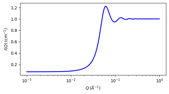
Fig. 130 1D plot corresponding to the default parameters of the model.

Source

hayter_msa.py \(\ \star\ \) hayter_msa.c

References

1. J B Hayter and J Penfold, Molecular Physics, 42 (1981) 109-118

2. J P Hansen and J B Hayter, Molecular Physics, 46 (1982) 651-656

3. M Kotlarchyk and S-H Chen, J. Chem. Phys., 79 (1983) 2461-2469

4. C G Malmberg and A A Maryott, J. Res. Nat. Bureau Standards, 56 (1956) 2641

Authorship and Verification

• Author:

• Last Modified by:

• Last Reviewed by: Steve King Date: March 28, 2019