multilayer_vesicle

Calculate form factor for a multi-lamellar vesicle

Parameter	Description	Units	Default value
scale	Scale factor or Volume fraction	None	1
background	Source background	cm-1	0.001
volfraction	volume fraction of vesicles	None	0.05
radius	radius of solvent filled core	Å	60
thick_shell	thickness of one shell	Å	10
thick_solvent	solvent thickness between shells	Å	10
sld_solvent	solvent scattering length density	10-6Å-2	6.4
sld	Shell scattering length density	10-6Å-2	0.4
n_shells	Number of shell plus solvent layer pairs (must be integer)	None	2

The returned value is scaled to units of cm^-1 sr^-1, absolute scale.

Definition

This model is a trivial extension of the core_shell_sphere function where the core is filled with solvent and is surrounded by \(N\) shells of material (such as lipids) interleaved with \(N - 1\) layers of solvent. For \(N = 1\), this returns the same as the vesicle model, except for the normalisation, which here is to outermost volume. The shell thicknesses and SLD are constant for all shells as expected for a multilayer vesicle.

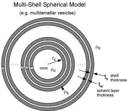
Fig. 83 Geometry of the multilayer_vesicle model.

See the core_shell_sphere model for more documentation.

The 1D scattering intensity is calculated in the following way (Guinier, 1955)

\[P(q) = \text{scale} \cdot \frac{\phi}{V(R_N)} F^2(q) + \text{background}\]

where

\[F(q) = (\rho_\text{shell}-\rho_\text{solv}) \sum_{i=1}^{N} \left[ 3V(r_i)\frac{\sin(qr_i) - qr_i\cos(qr_i)}{(qr_i)^3} - 3V(R_i)\frac{\sin(qR_i) - qR_i\cos(qR_i)}{(qR_i)^3} \right]\]

for

\[\begin{split}r_i &= r_c + (i-1)(t_s + t_w) \text{ solvent radius before shell } i \\ R_i &= r_i + t_s \text{ shell radius for shell } i\end{split}\]

\(\phi\) is the volume fraction of particles, \(V(r)\) is the volume of a sphere of radius \(r\), \(r_c\) is the radius of the core, \(t_s\) is the thickness of the shell, \(t_w\) is the thickness of the solvent layer between the shells, \(\rho_\text{shell}\) is the scattering length density of a shell, and \(\rho_\text{solv}\) is the scattering length density of the solvent.

USAGE NOTES

• The outer-most shell radius \(R_N\) is used as the effective radius for \(P(Q)\) when \(P(Q) * S(Q)\) is applied. calculations rather slow.

• The number of shells is always rounded to an integer value as a non integer number of layers is not physical.

• Thus polydispersity should only be applied to number of shells VERY CAREFULLY. A possible legitimate use would be for mixed systems in which some vesicles have 1 shell, some have 2, etc. A polydispersity on \(N\) can be used to model the data by using the “array distribution” feature. First create a file such as shell_dist.txt containing the relative portion of each vesicle size:

  1 20
  2  4
  3  1
  

  Turn on polydispersity and select an array distribution for the n_shells parameter. Choose the above shell_dist.txt file, and the model will be computed with 80% 1-shell vesicles, 16% 2-shell vesicles and 4% 3-shell vesicles.

• This is a highly non-linear, highly oscillatory (especially around the q-values that correspond to the repeat distance of the layers), model function complicated by the fact that the number of water/shell pairs must physically be an integer value, although the optimization treats it as a floating point value. Thus it may be that the resolution interpolation is not sufficiently fine grained in certain cases. Please report any such occurrences to the SasView team. Generally, for the best possible experience:

• Start with the best possible guess

• Using a priori knowledge, hold as many parameters fixed as possible

• if N=1, tw (water thickness) must by definition be zero. Both N and tw should be fixed during fitting.

• If N>1, use constraints to keep N > 1

• Because N only really moves in integer steps, it may get “stuck” if the optimizer step size is too small so care should be taken If you experience problems with this please contact the SasView team and let them know the issue preferably with example data and model which fail to converge.

The 2D scattering intensity is the same as 1D, regardless of the orientation of the q vector which is defined as:

\[q = \sqrt{q_x^2 + q_y^2}\]

For information about polarised and magnetic scattering, see the Polarisation/Magnetic Scattering documentation.

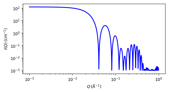
Fig. 84 1D plot corresponding to the default parameters of the model.

Source

multilayer_vesicle.py \(\ \star\ \) multilayer_vesicle.c \(\ \star\ \) sas_3j1x_x.c

References

1. B Cabane, Small Angle Scattering Methods, in Surfactant Solutions: New Methods of Investigation, Ch.2, Surfactant Science Series Vol. 22, Ed. R Zana and M Dekker, New York, (1987).

Authorship and Verification

• Author: NIST IGOR/DANSE Date: pre 2010

• Converted to sasmodels by: Piotr Rozyczko Date: Feb 24, 2016

• Last Modified by: Paul Kienzle Date: Feb 7, 2017

• Last Reviewed by: Steve King Date: March 28, 2019