parallelepiped¶

Rectangular parallelepiped with uniform scattering length density.

Parameter	Description	Units	Default value
scale	Scale factor or Volume fraction	None	1
background	Source background	cm^-1	0.001
sld	Parallelepiped scattering length density	10^-6Å^-2	4
sld_solvent	Solvent scattering length density	10^-6Å^-2	1
length_a	Shorter side of the parallelepiped	Å	35
length_b	Second side of the parallelepiped	Å	75
length_c	Larger side of the parallelepiped	Å	400
theta	c axis to beam angle	degree	60
phi	rotation about beam	degree	60
psi	rotation about c axis	degree	60

The returned value is scaled to units of cm^-1 sr^-1, absolute scale.

Definition

This model calculates the scattering from a rectangular solid (Fig. 69). If you need to apply polydispersity, see also rectangular_prism. For information about polarised and magnetic scattering, see the Polarisation/Magnetic Scattering documentation.

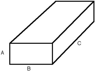
../../_images/parallelepiped_geometry.jpg — Fig. 69 Parallelepiped with the corresponding definition of sides.¶

The three dimensions of the parallelepiped (strictly here a cuboid) may be given in any size order as long as the particles are randomly oriented (i.e. take on all possible orientations see notes on 2D below). To avoid multiple fit solutions, especially with Monte-Carlo fit methods, it may be advisable to restrict their ranges. There may be a number of closely similar “best fits”, so some trial and error, or fixing of some dimensions at expected values, may help.

The form factor is normalized by the particle volume and the 1D scattering intensity \(I(q)\) is then calculated as:

\[I(q) = \frac{\text{scale}}{V} (\Delta\rho \cdot V)^2 \left< P(q, \alpha, \beta) \right> + \text{background}\]

where the volume \(V = A B C\), the contrast is defined as \(\Delta\rho = \rho_\text{p} - \rho_\text{solvent}\), \(P(q, \alpha, \beta)\) is the form factor corresponding to a parallelepiped oriented at an angle \(\alpha\) (angle between the long axis C and \(\vec q\)), and \(\beta\) (the angle between the projection of the particle in the \(xy\) detector plane and the \(y\) axis) and the averaging \(\left<\ldots\right>\) is applied over all orientations.

Assuming \(a = A/B < 1\), \(b = B /B = 1\), and \(c = C/B > 1\), the form factor is given by (Mittelbach and Porod, 1961 [1])

\[P(q, \alpha) = \int_0^1 \phi_Q\left(\mu \sqrt{1-\sigma^2},a\right) \left[S(\mu c \sigma/2)\right]^2 d\sigma\]

with

\[\begin{split}\phi_Q(\mu,a) &= \int_0^1 \left\{S\left[\frac{\mu}{2}\cos\left(\frac{\pi}{2}u\right)\right] S\left[\frac{\mu a}{2}\sin\left(\frac{\pi}{2}u\right)\right] \right\}^2 du \\ S(x) &= \frac{\sin x}{x} \\ \mu &= qB\end{split}\]

where substitution of \(\sigma = cos\alpha\) and \(\beta = \pi/2 \ u\) have been applied.

For oriented particles, the 2D scattering intensity, \(I(q_x, q_y)\), is given as:

\[I(q_x, q_y) = \frac{\text{scale}}{V} (\Delta\rho \cdot V)^2 P(q_x, q_y) + \text{background}\]

Where \(P(q_x, q_y)\) for a given orientation of the form factor is calculated as

\[P(q_x, q_y) = \left[\frac{\sin(\tfrac{1}{2}qA\cos\alpha)}{(\tfrac{1} {2}qA\cos\alpha)}\right]^2 \left[\frac{\sin(\tfrac{1}{2}qB\cos\beta)}{(\tfrac{1} {2}qB\cos\beta)}\right]^2 \left[\frac{\sin(\tfrac{1}{2}qC\cos\gamma)}{(\tfrac{1} {2}qC\cos\gamma)}\right]^2\]

with

\[\begin{split}\cos\alpha &= \hat A \cdot \hat q, \\ \cos\beta &= \hat B \cdot \hat q, \\ \cos\gamma &= \hat C \cdot \hat q\end{split}\]

FITTING NOTES

The 2nd virial coefficient of the parallelepiped is calculated based on the averaged effective radius, after appropriately sorting the three dimensions, to give an oblate or prolate particle, \((=\sqrt{AB/\pi})\) and length \((= C)\) values, and used as the effective radius for \(S(q)\) when \(P(q) \cdot S(q)\) is applied.
For 2d data the orientation of the particle is required, described using angles \(\theta\), \(\phi\) and \(\Psi\) as in the diagrams below, where \(\theta\) and \(\phi\) define the orientation of the director in the laboratory reference frame of the beam direction (\(z\)) and detector plane (\(x-y\) plane), while the angle \(\Psi\) is effectively the rotational angle around the particle \(C\) axis. For \(\theta = 0\) and \(\phi = 0\), \(\Psi = 0\) corresponds to the \(B\) axis oriented parallel to the y-axis of the detector with \(A\) along the x-axis. For other \(\theta\), \(\phi\) values, the order of rotations matters. In particular, the parallelepiped must first be rotated \(\theta\) degrees in the \(x-z\) plane before rotating \(\phi\) degrees around the \(z\) axis (in the \(x-y\) plane). Applying orientational distribution to the particle orientation (i.e jitter to one or more of these angles) can get more confusing as jitter is defined NOT with respect to the laboratory frame but the particle reference frame. It is thus highly recommended to read Oriented Particles for further details of the calculation and angular dispersions.

Note

For 2d, constraints must be applied during fitting to ensure that the order of sides chosen is not altered, and hence that the correct definition of angles is preserved. For the default choice shown here, that means ensuring that the inequality \(A < B < C\) is not violated, The calculation will not report an error, but the results may be not correct.

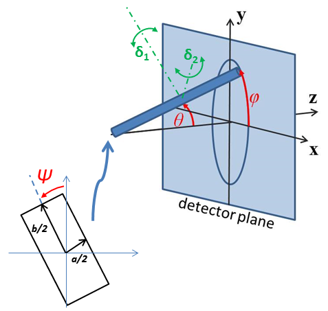
../../_images/parallelepiped_angle_definition.png — Fig. 70 Definition of the angles for oriented parallelepiped, shown with \(A<B<C\).¶

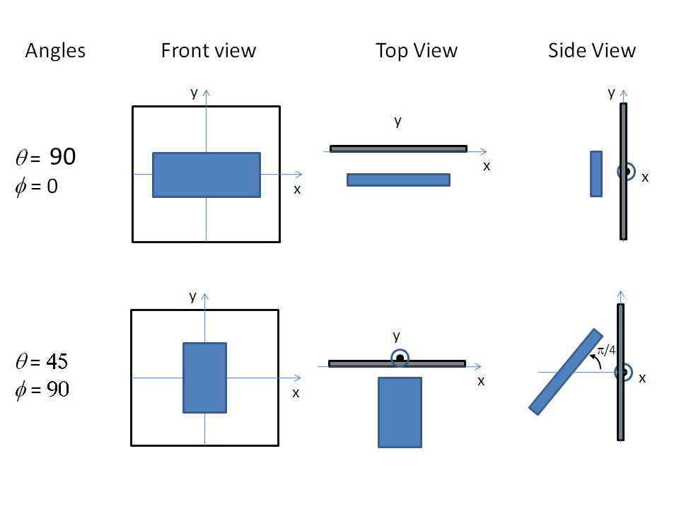
../../_images/parallelepiped_angle_projection.png — Fig. 71 Examples of the angles for an oriented parallelepiped against the detector plane.¶

Validation

Validation of the code was done by comparing the output of the 1D calculation to the angular average of the output of a 2D calculation over all possible angles.

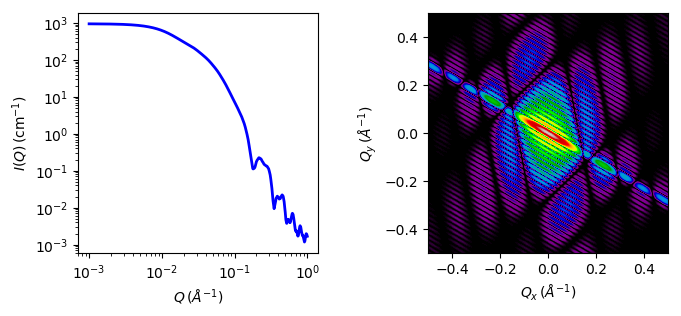
../../_images/parallelepiped_autogenfig.png — Fig. 72 1D and 2D plots corresponding to the default parameters of the model.¶

Source

parallelepiped.py \(\ \star\ \) parallelepiped.c \(\ \star\ \) gauss76.c

References

parallelepiped¶

Previous topic

Next topic

This Page

References

See also Nayuk [2] and Onsager [3].
Authorship and Verification
Author: NIST IGOR/DANSE Date: pre 2010
Last Modified by: Paul Kienzle Date: April 05, 2017
Last Reviewed by: Miguel Gonzales and Paul Butler Date: May 24, 2018 - documentation updated