spherical_sld

Spherical SLD intensity calculation

Parameter	Description	Units	Default value
scale	Scale factor or Volume fraction	None	1
background	Source background	cm-1	0.001
n_shells	number of shells (must be integer)	None	1
sld_solvent	solvent sld	10-6Å-2	1
sld[n_shells]	sld of the shell	10-6Å-2	4.06
thickness[n_shells]	thickness shell	Å	100
interface[n_shells]	thickness of the interface	Å	50
shape[n_shells]	interface shape	None	0
nu[n_shells]	interface shape exponent	None	2.5
n_steps	number of steps in each interface (must be an odd integer)	None	35

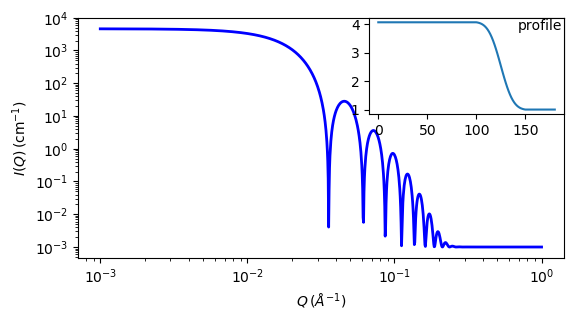
The returned value is scaled to units of cm^-1 sr^-1, absolute scale.

Definition

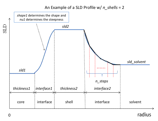
Similarly to the onion, this model provides the form factor, $P(q)$, for a multi-shell sphere, where the interface between the each neighboring shells can be described by the error function, power-law, or exponential functions. The scattering intensity is computed by building a continuous custom SLD profile along the radius of the particle. The SLD profile is composed of a number of uniform shells with interfacial shells between them.

Fig. 93 Example SLD profile

Unlike the onion model (using an analytical integration), the interfacial shells here are sub-divided and numerically integrated assuming each sub-shell is described by a line function, with n_steps sub-shells per interface. The form factor is normalized by the total volume of the sphere.

Note

n_shells must be an integer. n_steps must be an ODD integer.

Interface shapes are as follows:

0: erf($\nu z$)

1: Rpow($z^\nu$)

2: Lpow($z^\nu$)

3: Rexp($-\nu z$)

4: Lexp($-\nu z$)

5: Boucher ($(1-z^2)^(\nu/2-2)$)

The form factor $P(q)$ in 1D is calculated by [1]:

$$P(q) = \frac{f^2}{V_\text{particle}} \text{ where } f = f_\text{core} + \sum_{\text{inter}_i=0}^N f_{\text{inter}_i} + \sum_{\text{flat}_i=0}^N f_{\text{flat}_i} +f_\text{solvent}$$

For a spherically symmetric particle with a particle density $\rho_x(r)$ the sld function can be defined as:

$$f_x = 4 \pi \int_{0}^{\infty} \rho_x(r) \frac{\sin(qr)} {qr^2} r^2 dr$$

so that individual terms can be calculated as follows:

$$\begin{split}f_\text{core} &= 4 \pi \int_{0}^{r_\text{core}} \rho_\text{core} \frac{\sin(qr)} {qr} r^2 dr \\ &= 3 \rho_\text{core} V(r_\text{core}) \left[ \frac{\sin(qr_\text{core}) - qr_\text{core} \cos(qr_\text{core})} {qr_\text{core}^3} \right] \\ f_{\text{inter}_i} &= 4 \pi \int_{\Delta t_{ \text{inter}_i } } \rho_{ \text{inter}_i } \frac{\sin(qr)} {qr} r^2 dr \\ f_{\text{shell}_i} &= 4 \pi \int_{\Delta t_{ \text{inter}_i } } \rho_{ \text{flat}_i } \frac{\sin(qr)} {qr} r^2 dr \\ &= 3 \rho_{\text{flat}_i} V (r_{\text{inter}_i} + \Delta t_{\text{inter}_i}) \left[ \frac{\sin(qr_{\text{inter}_i} + \Delta t_{\text{inter}_i}) - q (r_{\text{inter}_i} + \Delta t_{ \text{inter}_i }) \cos(q(r_{\text{inter}_i} + \Delta t_{\text{inter}_i}))} {q ( r_{\text{inter}_i} + \Delta t_{\text{inter}_i} )^3 } \right] \\ &\quad {} - 3 \rho_{ \text{flat}_i } V (r_{\text{inter}_i}) \left[ \frac{\sin(qr_{\text{inter}_i}) - qr_{\text{flat}_i} \cos(qr_{\text{inter}_i})} {qr_{\text{inter}_i}^3} \right] \\ f_\text{solvent} &= 4 \pi \int_{r_N}^{\infty} \rho_\text{solvent} \frac{\sin(qr)} {qr} r^2 dr \\ &= 3 \rho_\text{solvent} V(r_N) \left[ \frac{\sin(qr_N) - qr_N \cos(qr_N)} {qr_N^3} \right]\end{split}$$

Here we assumed that the SLDs of the core and solvent are constant in $r$. The SLD at the interface between shells, $\rho_{\text {inter}_i}$ is calculated with a function chosen by an user, where the functions are

Exp:

$$\begin{split}\rho_{{inter}_i}(r) &= \begin{cases} B\, \exp\left( \frac{\pm A(r - r_{\text{flat}_i})}{\Delta t_{\text{inter}_i}} \right) + C & \mbox{for } A \neq 0 \\ B\, \left( \frac{(r - r_{\text{flat}_i})}{\Delta t_{\text{inter}_i}} \right) + C & \mbox{for } A = 0 \\ \end{cases}\end{split}$$

Power-Law:

$$\begin{split}\rho_{{inter}_i}(r) &= \begin{cases} \pm B\, \left( \frac{(r - r_{\text{flat}_i})}{\Delta t_{ \text{inter}_i }} \right) ^A + C & \mbox{for } A \neq 0 \\ \rho_{\text{flat}_{i+1}} & \mbox{for } A = 0 \\ \end{cases}\end{split}$$

Erf:

$$\begin{split}\rho_{{inter}_i}(r) = \begin{cases} B\, \text{erf} \left( \frac{A(r - r_{\text{flat}_i})}{\sqrt{2} \Delta t_{\text{inter}_i}} \right) + C & \mbox{for } A \neq 0 \\ B\, \left( \frac{(r - r_{\text{flat}_i})}{\Delta t_{\text{inter}_i}} \right) +C & \mbox{for } A = 0 \\ \end{cases}\end{split}$$

Boucher [2]:

$$\begin{split}\rho_{{inter}_i}(r) = \begin{cases} \pm B\, \left(1- (\frac{(r - r_{\text{flat}_i})}{\Delta t_{ \text{inter}_i }})^2 \right) ^(A/2-2) + C & \mbox{for } A \neq 0 \\ \rho_{\text{flat}_{i+1}} & \mbox{for } A = 0 \\ \end{cases}\end{split}$$

The functions are normalized so that they vary between 0 and 1, and they are constrained such that the SLD is continuous at the boundaries of the interface as well as each sub-shell. Thus B and C are determined.

Once $\rho_{\text{inter}_i}$ is found at the boundary of the sub-shell of the interface, we can find its contribution to the form factor $P(q)$

$$\begin{split}f_{\text{inter}_i} &= 4 \pi \int_{\Delta t_{\text{inter}_i} } \rho_{\text{inter}_i} \frac{\sin(qr)}{qr} r^2 dr \\ &= 4 \pi \sum_{j=1}^{n_\text{steps}} \int_{r_j}^{r_{j+1}} \rho_{\text{inter}_i}(r_j) \frac{\sin(qr)}{qr} r^2 dr \\ &\approx 4 \pi \sum_{j=1}^{n_\text{steps}} \Biggl[ 3 (\rho_{\text{inter}_i}(r_{j+1}) - \rho_{\text{inter}_i}(r_{j})) V (r_j) \left[ \frac{r_j^2 \beta_\text{out}^2 \sin(\beta_\text{out}) - (\beta_\text{out}^2-2) \cos(\beta_\text{out})} {\beta_\text{out}^4} \right] \\ &\quad {} - 3 (\rho_{\text{inter}_i}(r_{j+1}) - \rho_{\text{inter}_i}(r_{j})) V(r_{j-1}) \left[ \frac{r_{j-1}^2 \sin(\beta_\text{in}) - (\beta_\text{in}^2-2) \cos(\beta_\text{in})} {\beta_\text{in}^4} \right] \\ &\quad {} + 3 \rho_{\text{inter}_i}(r_{j+1}) V(r_j) \left[ \frac{\sin(\beta_\text{out}) - \cos(\beta_\text{out})} {\beta_\text{out}^4} \right] \\ &\quad {} - 3 \rho_{\text{inter}_i}(r_{j}) V(r_j) \left[ \frac{\sin(\beta_\text{in}) - \cos(\beta_\text{in})} {\beta_\text{in}^4} \right] \Biggr]\end{split}$$

where

$$\begin{align*} V(a) &= \frac {4\pi}{3}a^3 & {} & {} \\ a_\text{in} &\sim \frac{r_j}{r_{j+1} -r_j} & a_\text{out} &\sim \frac{r_{j+1}}{r_{j+1} -r_j} \\ \beta_\text{in} &= qr_j & \beta_\text{out} &= qr_{j+1} \end{align*}$$

We assume $\rho_{\text{inter}_j} (r)$ is approximately linear within the sub-shell $j$.

Finally the form factor can be calculated by

$$P(q) = \frac{[f]^2} {V_\text{particle}} \mbox{ where } V_\text{particle} = V(r_{\text{shell}_N})$$

For 2D data the scattering intensity is calculated in the same way as 1D, where the $q$ vector is defined as

$$q = \sqrt{q_x^2 + q_y^2}$$

Note

The outer most radius is used as the effective radius for $S(Q)$ when $P(Q) * S(Q)$ is applied.

Fig. 94 1D plot corresponding to the default parameters of the model.

Source

spherical_sld.py $\ \star\ $ spherical_sld.c $\ \star\ $ sas_3j1x_x.c $\ \star\ $ sas_erf.c $\ \star\ $ polevl.c

References

[1]

L A Feigin and D I Svergun, Structure Analysis by Small-Angle X-Ray and Neutron Scattering, Plenum Press, New York, (1987)

[2]

B Boucher, P Chieux, P Convert, and M Tournarie, Metal Physics, 13,1339 (1983).

Authorship and Verification

• Author: Jae-Hie Cho Date: Nov 1, 2010

• Last Modified by: Paul Kienzle Date: Dec 20, 2016

• Last Reviewed by: Steve King Date: March 29, 2019