Smearing Functions

Sometimes it will be necessary to correct reduced experimental data for the physical effects of the instrumental geometry in use. This process is called desmearing. However, calculated/simulated data - which by definition will be perfect/exact - can be smeared to make it more representative of what might actually be measured experimentally.

SasView provides the following three smearing algorithms:

• Slit Smearing
• Pinhole Smearing
• 2D Smearing

Slit Smearing

This type of smearing is normally only encountered with data from X-ray Kratky cameras or X-ray/neutron Bonse-Hart USAXS/USANS instruments.

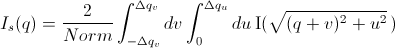
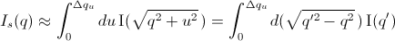
The slit-smeared scattering intensity is defined by

where Norm is given by

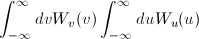
[Equation 1]

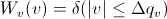
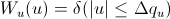
The functions and refer to the slit width weighting function and the slit height weighting determined at the given q point, respectively. It is assumed that the weighting function is described by a rectangular function, such that

[Equation 2]

and

[Equation 3]

so that for and u.

Here and stand for the slit height (FWHM/2) and the slit width (FWHM/2) in q space.

This simplifies the integral in Equation 1 to

[Equation 4]

which may be solved numerically, depending on the nature of and .

Solution 1

For = 0 and = constant.

For discrete q values, at the q values of the data points and at the q values extended up to q_N= q_i + the smeared intensity can be approximately calculated as

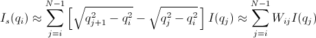
[Equation 5]

where = 0 for I_s when j < i or j > N-1.

Solution 2

For = constant and = 0.

Similar to Case 1

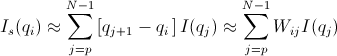for q_p = q_i - and q_N = q_i +

[Equation 6]

where = 0 for I_s when j < p or j > N-1.

Solution 3

For = constant and = constant.

In this case, the best way is to perform the integration of Equation 1 numerically for both slit height and slit width. However, the numerical integration is imperfect unless a large number of iterations, say, at least 10000 by 10000 for each element of the matrix W, is performed. This is usually too slow for routine use.

An alternative approach is used in SasView which assumes slit width << slit height. This method combines Solution 1 with the numerical integration for the slit width. Then

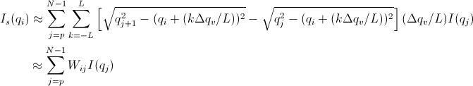
[Equation 7]

for q_p = q_i - and q_N = q_i +

where = 0 for I_s when j < p or j > N-1.

Pinhole Smearing

This is the type of smearing normally encountered with data from synchrotron SAXS cameras and SANS instruments.

The pinhole smearing computation is performed in a similar fashion to the slit- smeared case above except that the weight function used is a Gaussian. Thus Equation 6 becomes

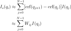
[Equation 8]

2D Smearing

The 2D smearing computation is performed in a similar fashion to the 1D pinhole smearing above except that the weight function used is a 2D elliptical Gaussian. Thus

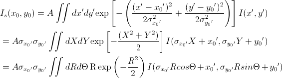
[Equation 9]

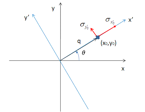
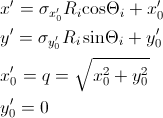
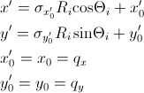
In Equation 9, x₀ = q cos(θ), y₀ = q sin(θ), and the primed axes, are all in the coordinate rotated by an angle θ about the z-axis (see the figure below) so that x’₀ = x₀ cos(θ) + y₀ sin(θ) and y’₀ = -x₀ sin(θ) + y₀ cos(θ). Note that the rotation angle is zero for a x-y symmetric elliptical Gaussian distribution. The A is a normalization factor.

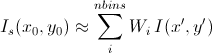
Now we consider a numerical integration where each of the bins in θ and R are evenly (this is to simplify the equation below) distributed by Δθ and ΔR, respectively, and it is further assumed that I(x’,y’) is constant within the bins. Then

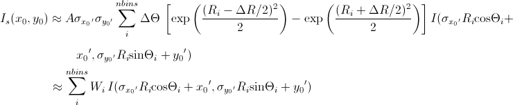
[Equation 10]

Since the weighting factor on each of the bins is known, it is convenient to transform x’-y’ back to x-y coordinates (by rotating it by -θ around the z axis).

Then, for a polar symmetric smear

[Equation 11]

where

while for a x-y symmetric smear

[Equation 12]

where

The current version of the SasView uses Equation 11 for 2D smearing, assuming that all the Gaussian weighting functions are aligned in the polar coordinate.

Weighting & Normalization

In all the cases above, the weighting matrix W is calculated on the first call to a smearing function, and includes ~60 q values (finely and evenly binned) below (>0) and above the q range of data in order to smear all data points for a given model and slit/pinhole size. The Norm factor is found numerically with the weighting matrix and applied on the computation of I_s.

Note

This help document was last changed by Steve King, 01May2015