hayter_msa

Hayter-Penfold rescaled MSA, charged sphere, interparticle S(Q) structure factor

Parameter	Description	Units	Default value
scale	Source intensity	None	1
background	Source background	cm-1	0.001
radius_effective	effective radius of charged sphere	Å	20.75
volfraction	volume fraction of spheres	None	0.0192
charge	charge on sphere (in electrons)	e	19
temperature	temperature, in Kelvin, for Debye length calculation	K	318.16
concentration_salt	conc of salt, moles/litre, 1:1 electolyte, for Debye length	M	0
dielectconst	dielectric constant (relative permittivity) of solvent, default water, for Debye length	None	71.08

The returned value is a dimensionless structure factor, \(S(q)\).

This calculates the structure factor (the Fourier transform of the pair correlation function \(g(r)\)) for a system of charged, spheroidal objects in a dielectric medium. When combined with an appropriate form factor (such as sphere, core+shell, ellipsoid, etc), this allows for inclusion of the interparticle interference effects due to screened coulomb repulsion between charged particles.

This routine only works for charged particles. If the charge is set to zero the routine may self-destruct! For non-charged particles use a hard sphere potential.

The salt concentration is used to compute the ionic strength of the solution which in turn is used to compute the Debye screening length. At present there is no provision for entering the ionic strength directly nor for use of any multivalent salts, though it should be possible to simulate the effect of this by increasing the salt concentration. The counterions are also assumed to be monovalent.

In sasview the effective radius may be calculated from the parameters used in the form factor \(P(q)\) that this \(S(q)\) is combined with.

The computation uses a Taylor series expansion at very small rescaled \(qR\), to avoid some serious rounding error issues, this may result in a minor artefact in the transition region under some circumstances.

For 2D data, the scattering intensity is calculated in the same way as 1D, where the \(q\) vector is defined as

\[q = \sqrt{q_x^2 + q_y^2}\]

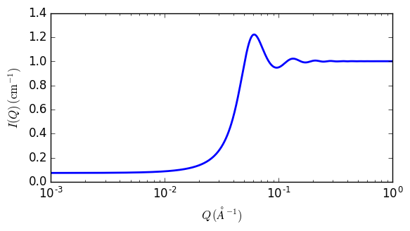
Fig. 111 1D plot corresponding to the default parameters of the model.

References

J B Hayter and J Penfold, Molecular Physics, 42 (1981) 109-118

J P Hansen and J B Hayter, Molecular Physics, 46 (1982) 651-656