spherical_sld
Sperical SLD intensity calculation
| Parameter |
Description |
Units |
Default value |
|---|
| scale |
Source intensity |
None |
1 |
| background |
Source background |
cm-1 |
0.001 |
| n_shells |
number of shells |
None |
1 |
| sld_solvent |
solvent sld |
10-6Å-2 |
1 |
| sld[n_shells] |
sld of the shell |
10-6Å-2 |
4.06 |
| thickness[n_shells] |
thickness shell |
Å |
100 |
| interface[n_shells] |
thickness of the interface |
Å |
50 |
| shape[n_shells] |
interface shape |
None |
0 |
| nu[n_shells] |
interface shape exponent |
None |
2.5 |
| n_steps |
number of steps in each interface (must be an odd integer) |
None |
35 |
The returned value is scaled to units of cm-1 sr-1, absolute scale.
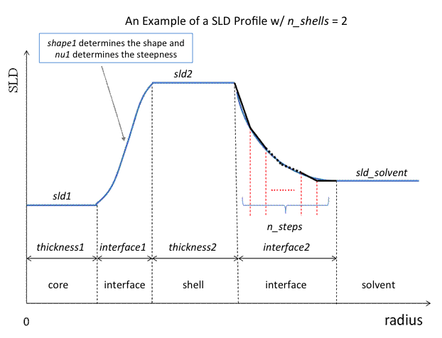
Similarly to the onion, this model provides the form factor, \(P(q)\), for
a multi-shell sphere, where the interface between the each neighboring
shells can be described by the error function, power-law, or exponential
functions. The scattering intensity is computed by building a continuous
custom SLD profile along the radius of the particle. The SLD profile is
composed of a number of uniform shells with interfacial shells between them.
Unlike the <onion> model (using an analytical integration), the interfacial
shells here are sub-divided and numerically integrated assuming each
sub-shell is described by a line function, with n_steps sub-shells per
interface. The form factor is normalized by the total volume of the sphere.
Interface shapes are as follows:
0: erf(|nu|*z)
1: Rpow(z^|nu|)
2: Lpow(z^|nu|)
3: Rexp(-|nu|z)
4: Lexp(-|nu|z)
Definition
The form factor \(P(q)\) in 1D is calculated by:
\[P(q) = \frac{f^2}{V_\text{particle}} \text{ where }
f = f_\text{core} + \sum_{\text{inter}_i=0}^N f_{\text{inter}_i} +
\sum_{\text{flat}_i=0}^N f_{\text{flat}_i} +f_\text{solvent}\]
For a spherically symmetric particle with a particle density \(\rho_x(r)\)
the sld function can be defined as:
\[f_x = 4 \pi \int_{0}^{\infty} \rho_x(r) \frac{\sin(qr)} {qr^2} r^2 dr\]
so that individual terms can be calculated as follows:
\[ \begin{align}\begin{aligned}f_\text{core} &= 4 \pi \int_{0}^{r_\text{core}} \rho_\text{core}
\frac{\sin(qr)} {qr} r^2 dr =
3 \rho_\text{core} V(r_\text{core})
\Big[ \frac{\sin(qr_\text{core}) - qr_\text{core} \cos(qr_\text{core})}
{qr_\text{core}^3} \Big]\\f_{\text{inter}_i} &= 4 \pi \int_{\Delta t_{ \text{inter}_i } }
\rho_{ \text{inter}_i } \frac{\sin(qr)} {qr} r^2 dr\\f_{\text{shell}_i} &= 4 \pi \int_{\Delta t_{ \text{inter}_i } }
\rho_{ \text{flat}_i } \frac{\sin(qr)} {qr} r^2 dr =
3 \rho_{ \text{flat}_i } V ( r_{ \text{inter}_i } +
\Delta t_{ \text{inter}_i } )
\Big[ \frac{\sin(qr_{\text{inter}_i} + \Delta t_{ \text{inter}_i } )
- q (r_{\text{inter}_i} + \Delta t_{ \text{inter}_i })
\cos(q( r_{\text{inter}_i} + \Delta t_{ \text{inter}_i } ) ) }
{q ( r_{\text{inter}_i} + \Delta t_{ \text{inter}_i } )^3 } \Big]
-3 \rho_{ \text{flat}_i } V(r_{ \text{inter}_i })
\Big[ \frac{\sin(qr_{\text{inter}_i}) - qr_{\text{flat}_i}
\cos(qr_{\text{inter}_i}) } {qr_{\text{inter}_i}^3} \Big]\\f_\text{solvent} &= 4 \pi \int_{r_N}^{\infty} \rho_\text{solvent}
\frac{\sin(qr)} {qr} r^2 dr =
3 \rho_\text{solvent} V(r_N)
\Big[ \frac{\sin(qr_N) - qr_N \cos(qr_N)} {qr_N^3} \Big]\end{aligned}\end{align} \]
Here we assumed that the SLDs of the core and solvent are constant in \(r\).
The SLD at the interface between shells, \(\rho_{\text {inter}_i}\)
is calculated with a function chosen by an user, where the functions are
Exp:
\[\begin{split}\rho_{{inter}_i} (r) &= \begin{cases}
B \exp\Big( \frac {\pm A(r - r_{\text{flat}_i})}
{\Delta t_{ \text{inter}_i }} \Big) +C & \mbox{for } A \neq 0 \\
B \Big( \frac {(r - r_{\text{flat}_i})}
{\Delta t_{ \text{inter}_i }} \Big) +C & \mbox{for } A = 0 \\
\end{cases}\end{split}\]
Power-Law
\[\begin{split}\rho_{{inter}_i} (r) &= \begin{cases}
\pm B \Big( \frac {(r - r_{\text{flat}_i} )} {\Delta t_{ \text{inter}_i }}
\Big) ^A +C & \mbox{for } A \neq 0 \\
\rho_{\text{flat}_{i+1}} & \mbox{for } A = 0 \\
\end{cases}\end{split}\]
Erf:
\[\begin{split}\rho_{{inter}_i} (r) = \begin{cases}
B \text{erf} \Big( \frac { A(r - r_{\text{flat}_i})}
{\sqrt{2} \Delta t_{ \text{inter}_i }} \Big) +C & \mbox{for } A \neq 0 \\
B \Big( \frac {(r - r_{\text{flat}_i} )} {\Delta t_{ \text{inter}_i }}
\Big) +C & \mbox{for } A = 0 \\
\end{cases}\end{split}\]
The functions are normalized so that they vary between 0 and 1, and they are
constrained such that the SLD is continuous at the boundaries of the interface
as well as each sub-shell. Thus B and C are determined.
Once \(\rho_{\text{inter}_i}\) is found at the boundary of the sub-shell of the
interface, we can find its contribution to the form factor \(P(q)\)
\[ \begin{align}\begin{aligned}f_{\text{inter}_i} &= 4 \pi \int_{\Delta t_{ \text{inter}_i } }
\rho_{ \text{inter}_i } \frac{\sin(qr)} {qr} r^2 dr =
4 \pi \sum_{j=1}^{n_\text{steps}}
\int_{r_j}^{r_{j+1}} \rho_{ \text{inter}_i } (r_j)
\frac{\sin(qr)} {qr} r^2 dr\\&\approx 4 \pi \sum_{j=1}^{n_\text{steps}} \Big[
3 ( \rho_{ \text{inter}_i } ( r_{j+1} ) - \rho_{ \text{inter}_i }
( r_{j} ) V (r_j)
\Big[ \frac {r_j^2 \beta_\text{out}^2 \sin(\beta_\text{out})
- (\beta_\text{out}^2-2) \cos(\beta_\text{out}) }
{\beta_\text{out}^4 } \Big]\\&{} - 3 ( \rho_{ \text{inter}_i } ( r_{j+1} ) - \rho_{ \text{inter}_i }
( r_{j} ) V ( r_{j-1} )
\Big[ \frac {r_{j-1}^2 \sin(\beta_\text{in})
- (\beta_\text{in}^2-2) \cos(\beta_\text{in}) }
{\beta_\text{in}^4 } \Big]\\&{} + 3 \rho_{ \text{inter}_i } ( r_{j+1} ) V ( r_j )
\Big[ \frac {\sin(\beta_\text{out}) - \cos(\beta_\text{out}) }
{\beta_\text{out}^4 } \Big]
- 3 \rho_{ \text{inter}_i } ( r_{j} ) V ( r_j )
\Big[ \frac {\sin(\beta_\text{in}) - \cos(\beta_\text{in}) }
{\beta_\text{in}^4 } \Big]
\Big]\end{aligned}\end{align} \]
where
\[\begin{align*}
V(a) &= \frac {4\pi}{3}a^3 && \\
a_\text{in} &\sim \frac{r_j}{r_{j+1} -r_j} \text{, } &a_\text{out}
&\sim \frac{r_{j+1}}{r_{j+1} -r_j} \\
\beta_\text{in} &= qr_j \text{, } &\beta_\text{out} &= qr_{j+1}
\end{align*}\]
We assume \(\rho_{\text{inter}_j} (r)\) is approximately linear
within the sub-shell \(j\).
Finally the form factor can be calculated by
\[P(q) = \frac{[f]^2} {V_\text{particle}} \mbox{ where } V_\text{particle}
= V(r_{\text{shell}_N})\]
For 2D data the scattering intensity is calculated in the same way as 1D,
where the \(q\) vector is defined as
\[q = \sqrt{q_x^2 + q_y^2}\]
Note
The outer most radius is used as the effective radius for \(S(Q)\)
when \(P(Q) * S(Q)\) is applied.
References
L A Feigin and D I Svergun, Structure Analysis by Small-Angle X-Ray
and Neutron Scattering, Plenum Press, New York, (1987)