stickyhardsphere

Sticky hard sphere structure factor, with Percus-Yevick closure

Parameter	Description	Units	Default value
scale	Source intensity	None	1
background	Source background	cm-1	0.001
radius_effective	effective radius of hard sphere	Å	50
volfraction	volume fraction of hard spheres	None	0.2
perturb	perturbation parameter, epsilon	None	0.05
stickiness	stickiness, tau	None	0.2

The returned value is a dimensionless structure factor, \(S(q)\).

This calculates the interparticle structure factor for a hard sphere fluid with a narrow attractive well. A perturbative solution of the Percus-Yevick closure is used. The strength of the attractive well is described in terms of “stickiness” as defined below.

The perturb (perturbation parameter), \(\epsilon\), should be held between 0.01 and 0.1. It is best to hold the perturbation parameter fixed and let the “stickiness” vary to adjust the interaction strength. The stickiness, \(\tau\), is defined in the equation below and is a function of both the perturbation parameter and the interaction strength. \(\tau\) and \(\epsilon\) are defined in terms of the hard sphere diameter \((\sigma = 2 R)\), the width of the square well, \(\Delta\) (same units as \(R\)), and the depth of the well, \(U_o\), in units of \(kT\). From the definition, it is clear that smaller \(\tau\) means stronger attraction.

\[\begin{split}\tau &= \frac{1}{12\epsilon} \exp(u_o / kT) \\ \epsilon &= \Delta / (\sigma + \Delta)\end{split}\]

where the interaction potential is

\[\begin{split}U(r) = \begin{cases} \infty & r < \sigma \\ -U_o & \sigma \leq r \leq \sigma + \Delta \\ 0 & r > \sigma + \Delta \end{cases}\end{split}\]

The Percus-Yevick (PY) closure was used for this calculation, and is an adequate closure for an attractive interparticle potential. This solution has been compared to Monte Carlo simulations for a square well fluid, with good agreement.

The true particle volume fraction, \(\phi\), is not equal to \(h\), which appears in most of the reference. The two are related in equation (24) of the reference. The reference also describes the relationship between this perturbation solution and the original sticky hard sphere (or adhesive sphere) model by Baxter.

NB: The calculation can go haywire for certain combinations of the input parameters, producing unphysical solutions - in this case errors are reported to the command window and the \(S(q)\) is set to -1 (so it will disappear on a log-log plot). Use tight bounds to keep the parameters to values that you know are physical (test them) and keep nudging them until the optimization does not hit the constraints.

In sasview the effective radius may be calculated from the parameters used in the form factor \(P(q)\) that this \(S(q)\) is combined with.

For 2D data the scattering intensity is calculated in the same way as 1D, where the \(q\) vector is defined as

\[q = \sqrt{q_x^2 + q_y^2}\]

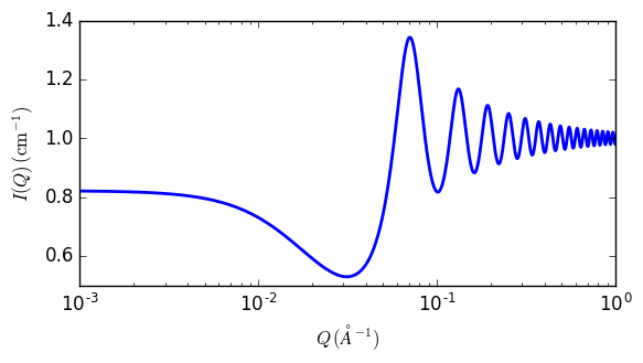
Fig. 113 1D plot corresponding to the default parameters of the model.

References

S V G Menon, C Manohar, and K S Rao, J. Chem. Phys., 95(12) (1991) 9186-9190