two_power_law

This model calculates an empirical functional form for SAS data characterized by two power laws.

Parameter	Description	Units	Default value
scale	Source intensity	None	1
background	Source background	cm-1	0.001
coefficent_1	coefficent A in low Q region	None	1
crossover	crossover location	Å-1	0.04
power_1	power law exponent at low Q	None	1
power_2	power law exponent at high Q	None	4

The returned value is scaled to units of cm^-1 sr^-1, absolute scale.

Definition

The scattering intensity \(I(q)\) is calculated as

\[\begin{split}I(q) = \begin{cases} A q^{-m1} + \text{background} & q <= q_c \\ C q^{-m2} + \text{background} & q > q_c \end{cases}\end{split}\]

where \(q_c\) = the location of the crossover from one slope to the other, \(A\) = the scaling coefficent that sets the overall intensity of the lower Q power law region, \(m1\) = power law exponent at low Q, and \(m2\) = power law exponent at high Q. The scaling of the second power law region (coefficent C) is then automatically scaled to match the first by following formula:

\[C = \frac{A q_c^{m2}}{q_c^{m1}}\]

Note

Be sure to enter the power law exponents as positive values!

For 2D data the scattering intensity is calculated in the same way as 1D, where the \(q\) vector is defined as

\[q = \sqrt{q_x^2 + q_y^2}\]

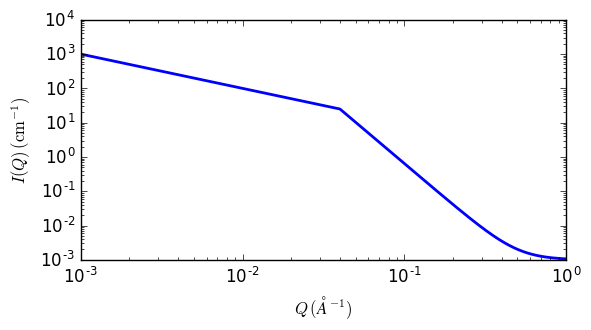
Fig. 108 1D plot corresponding to the default parameters of the model.

References

None.

Author: NIST IGOR/DANSE on: pre 2010

Last Modified by: Wojciech Wpotrzebowski on: February 18, 2016

Last Reviewed by: Paul Butler on: March 21, 2016