triaxial_ellipsoid

Ellipsoid of uniform scattering length density with three independent axes.

Parameter	Description	Units	Default value
scale	Source intensity	None	1
background	Source background	cm-1	0.001
sld	Ellipsoid scattering length density	10-6Å-2	4
sld_solvent	Solvent scattering length density	10-6Å-2	1
radius_equat_minor	Minor equatorial radius, Ra	Å	20
radius_equat_major	Major equatorial radius, Rb	Å	400
radius_polar	Polar radius, Rc	Å	10
theta	polar axis to beam angle	degree	60
phi	rotation about beam	degree	60
psi	rotation about polar axis	degree	60

The returned value is scaled to units of cm^-1 sr^-1, absolute scale.

Definition

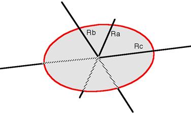
Fig. 42 Ellipsoid with \(R_a\) as radius_equat_minor, \(R_b\) as radius_equat_major and \(R_c\) as radius_polar.

Given an ellipsoid

\[\frac{X^2}{R_a^2} + \frac{Y^2}{R_b^2} + \frac{Z^2}{R_c^2} = 1\]

the scattering for randomly oriented particles is defined by the average over all orientations \(\Omega\) of:

\[P(q) = \text{scale}(\Delta\rho)^2\frac{V}{4 \pi}\int_\Omega\Phi^2(qr)\,d\Omega + \text{background}\]

where

\[\begin{split}\Phi(qr) &= 3 j_1(qr)/qr = 3 (\sin qr - qr \cos qr)/(qr)^3 \\ r^2 &= R_a^2e^2 + R_b^2f^2 + R_c^2g^2 \\ V &= \tfrac{4}{3} \pi R_a R_b R_c\end{split}\]

The \(e\), \(f\) and \(g\) terms are the projections of the orientation vector on \(X\), \(Y\) and \(Z\) respectively. Keeping the orientation fixed at the canonical axes, we can integrate over the incident direction using polar angle \(-\pi/2 \le \gamma \le \pi/2\) and equatorial angle \(0 \le \phi \le 2\pi\) (as defined in ref [1]),

\[\langle\Phi^2\rangle = \int_0^{2\pi} \int_{-\pi/2}^{\pi/2} \Phi^2(qr) \cos \gamma\,d\gamma d\phi\]

with \(e = \cos\gamma \sin\phi\), \(f = \cos\gamma \cos\phi\) and \(g = \sin\gamma\). A little algebra yields

\[r^2 = b^2(p_a \sin^2 \phi \cos^2 \gamma + 1 + p_c \sin^2 \gamma)\]

for

\[p_a = \frac{a^2}{b^2} - 1 \text{ and } p_c = \frac{c^2}{b^2} - 1\]

Due to symmetry, the ranges can be restricted to a single quadrant \(0 \le \gamma \le \pi/2\) and \(0 \le \phi \le \pi/2\), scaling the resulting integral by 8. The computation is done using the substitution \(u = \sin\gamma\), \(du = \cos\gamma\,d\gamma\), giving

\[\begin{split}\langle\Phi^2\rangle &= 8 \int_0^{\pi/2} \int_0^1 \Phi^2(qr) du d\phi \\ r^2 &= b^2(p_a \sin^2(\phi)(1 - u^2) + 1 + p_c u^2)\end{split}\]

Though for convenience we describe the three radii of the ellipsoid as equatorial and polar, they may be given in \(any\) size order. To avoid multiple solutions, especially with Monte-Carlo fit methods, it may be advisable to restrict their ranges. For typical small angle diffraction situations there may be a number of closely similar “best fits”, so some trial and error, or fixing of some radii at expected values, may help.

To provide easy access to the orientation of the triaxial ellipsoid, we define the axis of the cylinder using the angles \(\theta\), \(\phi\) and \(\psi\). These angles are defined analogously to the elliptical_cylinder below, note that angle \(\phi\) is now NOT the same as in the equations above.

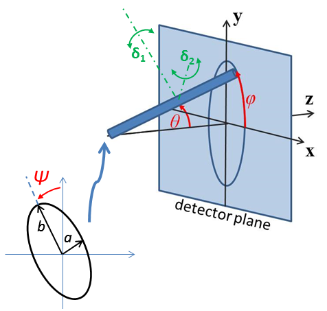
Fig. 43 Definition of angles for oriented triaxial ellipsoid, where radii are for illustration here \(a < b << c\) and angle \(\Psi\) is a rotation around the axis of the particle.

For oriented ellipsoids the theta, phi and psi orientation parameters will appear when fitting 2D data, see the elliptical_cylinder model for further information.

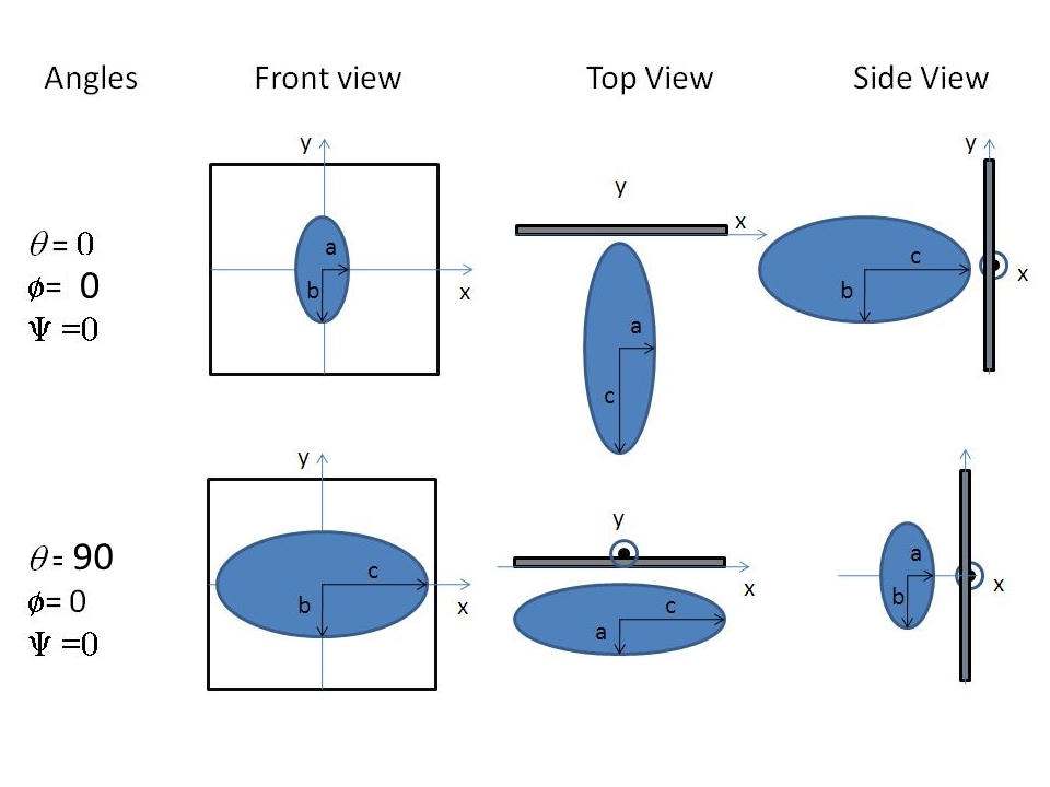
Fig. 44 Some examples for an oriented triaxial ellipsoid.

The radius-of-gyration for this system is \(R_g^2 = (R_a R_b R_c)^2/5\).

The contrast \(\Delta\rho\) is defined as SLD(ellipsoid) - SLD(solvent). In the parameters, \(R_a\) is the minor equatorial radius, \(R_b\) is the major equatorial radius, and \(R_c\) is the polar radius of the ellipsoid.

NB: The 2nd virial coefficient of the triaxial solid ellipsoid is calculated after sorting the three radii to give the most appropriate prolate or oblate form, from the new polar radius \(R_p = R_c\) and effective equatorial radius, \(R_e = \sqrt{R_a R_b}\), to then be used as the effective radius for \(S(q)\) when \(P(q) \cdot S(q)\) is applied.

Validation

Validation of our code was done by comparing the output of the 1D calculation to the angular average of the output of 2D calculation over all possible angles.

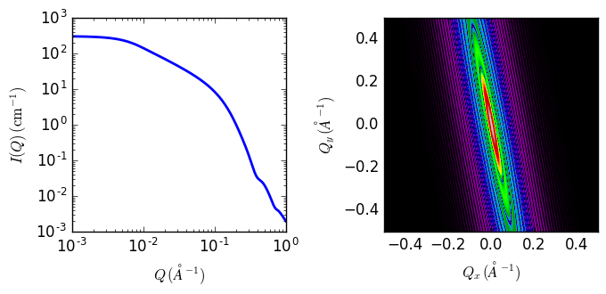
Fig. 45 1D and 2D plots corresponding to the default parameters of the model.

References

[1] Finnigan, J.A., Jacobs, D.J., 1971. Light scattering by ellipsoidal particles in solution, J. Phys. D: Appl. Phys. 4, 72-77. doi:10.1088/0022-3727/4/1/310

Authorship and Verification

• Author: NIST IGOR/DANSE Date: pre 2010
• Last Modified by: Paul Kienzle (improved calculation) Date: April 4, 2017
• Last Reviewed by: Paul Kienzle & Richard Heenan Date: April 4, 2017