Invariant Calculation
Principle
In a multi-phase system, the integral of the appropriately dimensionally-weighted scattering cross-section (ie, ‘intensity’, \(I(Q)\)) is a constant directly proportional to the mean-square average fluctuation in scattering length density (SLD) and the phase composition but which, usefully, is independent of the shape of the phase domains. If the scattering cross-section data are in absolute units this constant is known as the Scattering Invariant, the Porod Invariant, or simply as the Invariant, \(Q^*\).
Note
In this document we shall denote the invariant by the often encountered symbol \(Q^*\). But the reader should be aware that other symbols can be encountered in the literature. Glatter & Kratky, and Stribeck, for example, both use \(Q\), the same symbol we use to denote the scattering vector in SasView(!), whilst Melnichenko uses \(Z\). Other variations include \(Q_I\).
If the data is measured on an instrument with ‘classic’ pinhole geometry then
whereas if the data is measured on an instrument with slit geometry
where \(\Delta Q_v\) is the slit height and \(Q\) denotes the scattering vector.
The worth of \(Q^*\) is that it can be used to determine quantities such as the volume fraction, composition, or specific surface area of a sample. It can also be used to cross-calibrate different SAS instruments.
The difficulty with using \(Q^*\) arises from the fact that experimental data is never measured over the range \(0 \le Q \le \infty\). At best, combining USAS and WAS data might cover the range \(10^{-5} \le Q \le 10\) \(Ang^{-1}\) . Thus, it is usually necessary to extrapolate the experimental data to both low and high \(Q\). For the
Low-\(Q\) region (<= \(Q_{min}\) in data):
- The Guinier function \(I_0.exp(-Q^2 R_g^2/3)\) can be used, where \(I_0\) and \(R_g\) are obtained by fitting the data within the range \(Q_{i}\) to \(Q_{i+j}\) (where \(i+j > i\)) at the lowest \(Q\)-values. Alternatively a power law can be used. Because the integrals above are weighted by \(Q^2\) or \(Q\) the low-\(Q\) extrapolation only contributes a small proportion, say <3%, to the value of \(Q^*\).
High-\(Q\) region (>= \(Q_{max}\) in data):
- The power law function \(C_p/Q^4\) is used where the constant \(C_p\) is obtained by fitting the data within the range \(Q_{n-m}\) to \(Q_n\) (where \(n-m < n\)) at the highest \(Q\)-values. This extrapolation typically contributes 3 - 20% of the value of \(Q^*\) so having data measured to as large a value of \(Q_{max}\) as possible is much more important.
Parameters
For a two-phase system, the most commonly encountered situation, the Invariant is
where \(\Delta\rho = (\rho_1 - \rho_2)\) is the SLD contrast and \(\phi_1\) and \(\phi_2\) are the volume fractions of the two phases (\(\phi_1 + \phi_2 = 1\)). From this the volume fraction, specific surface area, and mean-square average SLD fluctuation can be determined.
Volume Fraction
and thus
Specific Surface Area
From Porod’s Law
where the Porod Constant is
and \(S_v\) is the specific surface area (the surface area-to-volume ratio, \(S/V\)). From this it follows that
SLD Fluctuation
The mean-square average of the SLD fluctuation is
where
Three-Phase Systems
For the extension of Invariant Analysis to three phases, see the Melnichenko reference, Chapter 6, Section 6.9.
Using invariant analysis
Load some data with the Data Explorer.
Select a dataset and use the Send To button on the Data Explorer to load the dataset into the Invariant panel. Or select Invariant from the Analysis category in the menu bar.
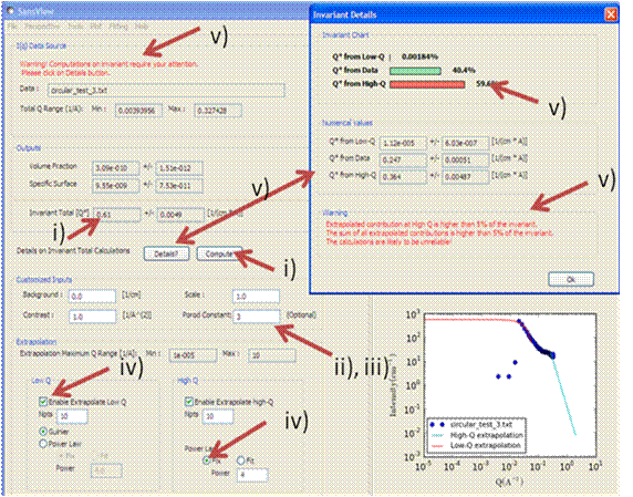
A first estimate of \(Q^*\) should be computed automatically. If not, click on the Compute button.
Use the Customised Inputs boxes on the Invariant panel to subtract any background, specify the contrast (i.e. difference in SLDs: note this must be specified for the eventual value of \(Q^*\) to be on an absolute scale and to therefore have any meaning), or to rescale the data.
(Optional) If known, a value for \(C_p\) can also be specified.
Adjust the extrapolation ranges and extrapolation types as necessary. In most cases the default values will suffice. Click the Compute button.
To adjust the lower and/or higher \(Q\) ranges, check the relevant Enable Extrapolate check boxes.
If power law extrapolations are chosen, the exponent can be either held fixed or fitted. The number of points, \(Npts\), to be used for the basis of the extrapolation can also be specified.
If the value of \(Q^*\) calculated with the extrapolated regions is invalid, a red warning will appear at the top of the Invariant panel.
The details of the calculation are available by clicking the Details button in the middle of the panel.
References
O. Glatter and O. Kratky Chapter 2 and Chapter 14 in Small Angle X-Ray Scattering Academic Press, New York, 1982
Available at: http://web.archive.org/web/20110824105537/http://physchem.kfunigraz.ac.at/sm/Service/Glatter_Kratky_SAXS_1982.zip
N. Stribeck Chapter 8 in X-Ray Scattering of Soft Matter Springer, 2007
Y.B. Melnichenko Chapter 6 in Small-Angle Scattering from Confined and Interfacial Fluids Springer, 2016
Note
This help document was last changed by Steve King, 10Jan2020