bcc_paracrystal

Body-centred cubic lattic with paracrystalline distortion

Parameter	Description	Units	Default value
scale	Scale factor or Volume fraction	None	1
background	Source background	cm-1	0.001
dnn	Nearest neighbour distance	Å	220
d_factor	Paracrystal distortion factor	None	0.06
radius	Particle radius	Å	40
sld	Particle scattering length density	10-6Å-2	4
sld_solvent	Solvent scattering length density	10-6Å-2	1
theta	c axis to beam angle	degree	60
phi	rotation about beam	degree	60
psi	rotation about c axis	degree	60

The returned value is scaled to units of cm^-1 sr^-1, absolute scale.

Definition

Calculates the scattering from a body-centered cubic lattice with paracrystalline distortion. Thermal vibrations are considered to be negligible, and the size of the paracrystal is infinitely large. Paracrystalline distortion is assumed to be isotropic and characterized by a Gaussian distribution.

The scattering intensity \(I(q)\) is calculated as

\[I(q) = \frac{\text{scale}}{V_p} V_\text{lattice} P(q) Z(q) + \text{background}\]

where scale is the volume fraction of crystal in the sample volume, \(V_\text{lattice}\) is the volume fraction of spheres in the crystal, \(V_p\) is the volume of the primary particle, \(P(q)\) is the form factor of the sphere (normalized), and \(Z(q)\) is the paracrystalline structure factor for a body-centered cubic structure.

Note

At this point the GUI does not return \(V_\text{lattice}\) separately so that the user will need to calculate it from the equation given and the appropriate returned parameters.

Warning

As per the equations below, this model will return I(q)=0 for all q if the distortion factor is equal to 0. The model is not meant to support perfect crystals.

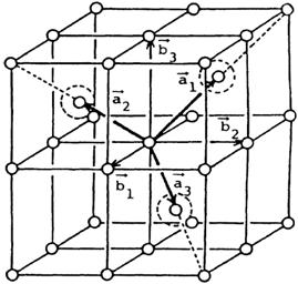
Fig. 51 Body-centered cubic (BCC) lattice taken from reference [1].

Following the derivation from reference [1], as corrected in reference [2], and based on the above figure, the primitive unit cell vectors \(\vec{a_1},\vec{a_2}\), and \(\vec{a_3}\), which enclose the smallest possible unit cell for the bcc lattice, are defined below:

\[\begin{split}\vec{a_1} &= \frac{1}{2}(-\vec{b_1} + \vec{b_2} + \vec{b_3}) \\ \vec{a_2} &= \frac{1}{2} (\vec{b_1} - \vec{b_2} + \vec{b_3}) \\ \vec{a_3} &= \frac{1}{2}(\vec{b_1} + \vec{b_2} -\vec{b_3}).\end{split}\]

where \(\vec{b_1},\vec{b_2}\), and \(\vec{b_3}\) are the unit cell vectors of the conventional unit cell, which is a unit cell that includes the full symmetry of the lattice. As defined by reference [1], the constant \(a\) is the lattice parameter of the conventional unit cell with \(|\vec{b_1}|=|\vec{b_2}|=|\vec{b_3}|=a\). Using this definition, the nearest-neighbor distance (\(D\)) is given by \(D=|\vec{a_1}|=|\vec{a_2}|=|\vec{a_3}|=\sqrt{(a/2)^2+(a/2)^2+(a/2)^2}=\sqrt{\frac{3a^2}{4}}=\frac{\sqrt{3}a}{2}\).

The volume of the primitive unit cell \(V_u\) is then given by:

\[\begin{split}V_u &= |(\vec{a_1}\times \vec{a_2})\cdot\vec{a_3}|\\ &= (\frac{a^2}{2},\frac{a^2}{2},0)\cdot(\frac{a}{2},\frac{a}{2},-\frac{a}{2})\\ &= a^3/2\end{split}\]

In this case, the volume fraction (\(V_{lattice}\)) of spherical particles with radius \(R\) sitting on the bcc lattice is given by:

\[\begin{split}V_{lattice} &= \frac{4/3 \pi R^3}{a^3/2}\\ &= \frac{8\pi R^3}{3a^3}\\ &= \frac{\sqrt{3} \pi R^3}{D^3}\end{split}\]

Now, continuing to follow [1], the structure (lattice) factor \(Z(\vec{q})\) for a 3D paracrystal can be written as:

\[Z(\vec{q}) = \prod_{k=1}^{3}Z_k(\vec{q})\]

with

\[Z_k(\vec{q}) = \frac{1-|F_k|^2}{1-2|F_k|\cos(\vec{a_k}\cdot\vec{q})+|F_k|^2}\]

and where \(F_k(\vec{q})\) is the structure factor of the primitive unit cell defined as:

\[F_k(\vec{q}) = e^{-\frac{1}{2} \Delta a^2_k q^2} \times e^{-i\vec{q}\cdot\vec{a_k}}.\]

Here, \(\vec{a_k}\) are the primitive unit cell vectors \(\vec{a_1}\), \(\vec{a_2}\), and \(\vec{a_3}\). Furthermore, \(\Delta a_k\) is the isotropic distortion of the lattice point from its ideal position and can be defined by a constant factor \(g=\Delta a / |\vec{a_1}| = \Delta a / |\vec{a_2}| = \Delta a / |\vec{a_3}|=\Delta a/D\).

Finally, assuming the definitions presented in this document, the authors of reference [1] have derived the lattice factors which are given by:

\[\begin{split}Z_1(q,\theta,\phi)&=[1-e^{-q^2\Delta a^2}]/\{1-2e^{-\frac{1}{2}q^2\Delta a^2}\cos[\frac{qa}{2}(\sin\theta \cos\phi + \sin\theta \sin\phi + \cos\theta)] + e^{-q^2\Delta a^2}\}\\ Z_2(q,\theta,\phi)&=[1-e^{-q^2\Delta a^2}]/\{1-2e^{-\frac{1}{2}q^2\Delta a^2}\cos[\frac{qa}{2}(-\sin\theta \cos\phi - \sin\theta \sin\phi + \cos\theta)] + e^{-q^2\Delta a^2}\}\\ Z_3(q,\theta,\phi)&=[1-e^{-q^2\Delta a^2}]/\{1-2e^{-\frac{1}{2}q^2\Delta a^2}\cos[\frac{qa}{2}(-\sin\theta \cos\phi + \sin\theta \sin\phi - \cos\theta)] + e^{-q^2\Delta a^2}\}\\\end{split}\]

Note that Sasview is using the nearest-neighbor parameter (\(D\)) as an input instead of the conventional unit cell parameter \(a\). In this case, using \(a=\frac{2D}{\sqrt{3}}\), we rewrite \(Z_1(q)\), \(Z_2(q)\), and \(Z_3(q)\) in terms of \(D\) instead of \(a\), which leads to:

\[\begin{split}Z_1(q,\theta,\phi)&=[1-e^{-q^2\Delta a^2}]/\{1-2e^{-\frac{1}{2}q^2\Delta a^2}\cos[\frac{qD}{\sqrt{3}}(\sin\theta \cos\phi + \sin\theta \sin\phi + \cos\theta)] + e^{-q^2\Delta a^2}\}\\ Z_2(q,\theta,\phi)&=[1-e^{-q^2\Delta a^2}]/\{1-2e^{-\frac{1}{2}q^2\Delta a^2}\cos[\frac{qD}{\sqrt{3}}(-\sin\theta \cos\phi - \sin\theta \sin\phi + \cos\theta)] + e^{-q^2\Delta a^2}\}\\ Z_3(q,\theta,\phi)&=[1-e^{-q^2\Delta a^2}]/\{1-2e^{-\frac{1}{2}q^2\Delta a^2}\cos[\frac{qD}{\sqrt{3}}(-\sin\theta \cos\phi + \sin\theta \sin\phi - \cos\theta)] + e^{-q^2\Delta a^2}\}\\\end{split}\]

Finally note that the position of the Bragg peaks for the bcc lattice are indexed by (reduced q-values):

\[\frac{qa}{2\pi}=\frac{qD}{\sqrt{3}\pi}=\sqrt{h^2+k^2+l^2}.\]

In the above equation, we used the conventional unit cell so not all permutations of h,k, and l will produce Bragg peaks. The Bragg scattering condition for bcc imposes that h+k+l = even. Thus the peak positions correspond to (just the first 5)

\[\begin{split}\begin{array}{lccccc} q/q_o & 1 & \sqrt{2} & \sqrt{3} & \sqrt{4} & \sqrt{5} \\ \text{Indices} & (110) & (200) & (211) & (220) & (310) \\ \end{array}\end{split}\]

Note

The calculation of \(Z(q)\) is a double numerical integral that must be carried out with a high density of points to properly capture the sharp peaks of the paracrystalline scattering. So be warned that the calculation is slow. Fitting of any experimental data must be resolution smeared for any meaningful fit. This makes a triple integral which may be very slow. If a double-precision GPU with OpenCL support is available this may improve the speed of the calculation.

This example dataset is produced using 200 data points, qmin = 0.001 Å^-1, qmax = 0.1 Å^-1 and the above default values.

The 2D (Anisotropic model) is based on the reference below where \(I(q)\) is approximated for 1d scattering. Thus the scattering pattern for 2D may not be accurate, particularly at low \(q\). For general details of the calculation and angular dispersions for oriented particles see Oriented Particles. Note that we are not responsible for any incorrectness of the 2D model computation.

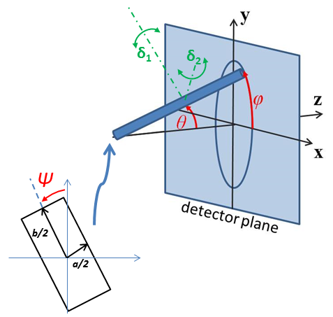
Fig. 52 Orientation of the crystal with respect to the scattering plane, when \(\theta = \phi = 0\) the \(c\) axis is along the beam direction (the \(z\) axis).

Fig. 53 1D and 2D plots corresponding to the default parameters of the model.

Source

bcc_paracrystal.py \(\ \star\ \) bcc_paracrystal.c \(\ \star\ \) sphere_form.c \(\ \star\ \) gauss150.c \(\ \star\ \) sas_3j1x_x.c

References

[1] (1,2,3,4,5)

Hideki Matsuoka et. al. Physical Review B, 36 (1987) 1754-1765 (Original Paper)

[2]

Hideki Matsuoka et. al. Physical Review B, 41 (1990) 3854-3856 (Corrections to FCC and BCC lattice structure calculation)

Authorship and Verification

• Author: NIST IGOR/DANSE Date: pre 2010

• Last Modified by: Jonathan Gaudet Date: September 26, 2022

• Last Reviewed by: Paul Butler Date: November 2, 2022