two_yukawa
User model for two Yukawa structure factor (S(q))
Parameter |
Description |
Units |
Default value |
|---|---|---|---|
radius_effective |
Å |
50 |
|
volfraction |
None |
0.1 |
|
k1 |
None |
6 |
|
k2 |
None |
-2 |
|
z1 |
None |
10 |
|
z2 |
None |
2 |
The returned value is a dimensionless structure factor, \(S(q)\).
This model calculates the structure factor, \(S(q)\), of one-component liquid systems interacting with a two-term Yukawa potential with the mean spherical approximation (MSA) by solving the Ornstein-Zernike (OZ) equation. Both Yukawa terms can be used to simulate either a repulsive or an attraction potential feature. For example, if one Yukawa term is chosen to be an attractive potential and the other a repulsive potential, the two Yukawa potential can simulate a potential with both a short-range attraction and long-range repulsion (SALR).[1,2] When combined with an appropriate form factor \(P(q)\), this allows for inclusion of the interparticle interference effects due to a relatively complex potential.
The algorithm used in this model was originally proposed and developed by Liu et al. in 2005 and implemented using MatLab.[1] This algorithm used a theory proposed by Hoye and Blum in 1977,[4] in which the structure factor is solved by using Baxter’s Q-method with the MSA closure.
The interaction potential \(V(r)\) is
where \(r\) is the normalized distance, \(\frac{r_{cc}}{2R}\). (\(R\) is the effective radius and \(r_{cc}\) is the distance between the center-of-mass of particles.) \(K_1\) and \(K_2\) are positive for repulsion and negative for attraction. \(Z_1\) and \(Z_2\) are the inversely proportional to the decay rate of the potential. They should always be positive.
To reduce numerical issues during fitting, the lower boundary of the absolute values for \(K_1\) and \(K_2\) are set to 0.0001. That is, when \(|K| < 0.0001\) it is adjusted 0.0001 while preserving the sign. Similarly, when \(Z_1\) or \(Z_2\) are less than 0.01, they are adjusted to 0.01. To make the two Yukawa terms functionally different, \(Z_1\) is adjusted to \(Z_2+0.01\) if the difference between them is less than 0.01. The impact of these changes on the accuracy of \(S(Q)\) was negligible for all tested cases. The algorithm works best if \(Z_1>Z_2\), particularly for large \(Z\) such as \(Z>20\). When \(Z_1\) is less than \(Z_2\), the code will automatically swap \(Z_1\) and \(Z_2\), and \(K_1\) and \(K_2\). \(S(Q)\) is set to 1.0 for volume fraction \(\phi < 10^{-10}\).
Note
The so-called \(\beta(q)\) (“beta”) approximation [3] can be used to calculate the effective structure factor for polydispersity and non-sphericity when a system is not too far away from the mono-disperse spherical systems.
In general, any closure used to solve the OZ equation is an approximation. Thus, the structure factor calculated using a closure is an approximation of the real structure factor. Its accuracy varies for different parameter ranges. One should not “blindly” trust the results. In addition, when using the O-Z equation to obtain the structure factor, it assumes that a system is in a liquid state. However, when the attraction potential is too strong the system may not be in a simple liquid state, and the OZ equation may not have a solution, or the solution may be unphysical.
Accuracy for the MSA closure used here to solve the OZ equation for two Yukawa potential was evaluated by Broccio, et al.[2] When the overall attraction is moderate, this algorithm produces reasonably accurate results. However, when the net attraction is very strong, it has been shown that the fitting algorithm tends to overestimate the attraction strength. Care is needed when discussing quantitative fitting results for those systems.
When the interaction distances \(Z_1\) and \(Z_2\) are large, the method implemented here may be influenced by the numerical accuracy of a computer. In general, when \(Z<20\), the code should function well for most cases. When \(Z>25\), sometimes the intermediate results of this code may run into the limit of the largest number that a computer can handle. Therefore, results may potentially become less reliable. Hence, the check of \(g(r)\) becomes very important in those situations. So far, no limitation of the value of \(K\) has been encountered except that they cannot be zero.
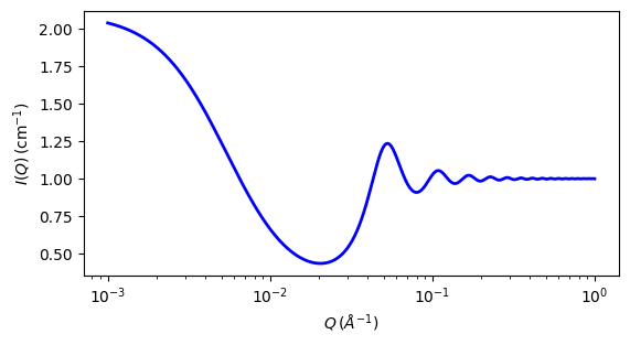
Fig. 133 1D plot corresponding to the default parameters of the model.
Source
References
Liu, W. R. Chen, S-H Chen, J. Chem. Phys., 122 (2005) 044507
Broccio, D. Costa, Y. Liu, S-H Chen, J. Chem. Phys., 124 (2006) 084501
Kotlarchyk and S-H Chen, J. Chem. Phys., 79 (1983) 2461-2469
Hoye, L. Blum, J. Stat. Phys., 16(1977) 399-413
Authorship and Verification
Author: Yun Liu Date: January 22, 2024
Last Modified by: Yun Liu Date: January 22, 2024
Last Reviewed by: Yun Liu Date: January 22, 2024