unified_power_Rg

Unified Power Rg

Parameter	Description	Units	Default value
scale	Scale factor or Volume fraction	None	1
background	Source background	cm-1	0.001
level	Level number	None	1
rg[level]	Radius of gyration	Å	15.8
power[level]	Power	None	4
B[level]		cm-1	4.5e-06
G[level]		cm-1	400

The returned value is scaled to units of cm^-1 sr^-1, absolute scale.

Definition

This model employs the empirical multiple level unified Exponential/Power-law fit method developed by Beaucage. Four functions are included so that 1, 2, 3, or 4 levels can be used. In addition a 0 level has been added which simply calculates

\[I(q) = \text{scale} / q + \text{background}\]

The Beaucage method is able to reasonably approximate the scattering from many different types of particles, including fractal clusters, random coils (Debye equation), ellipsoidal particles, etc.

The model works best for mass fractal systems characterized by Porod exponents between 5/3 and 3. It should not be used for surface fractal systems. Hammouda (2010) has pointed out a deficiency in the way this model handles the transitioning between the Guinier and Porod regimes and which can create artefacts that appear as kinks in the fitted model function.

Also see the guinier_porod model.

The empirical fit function is:

\[I(q) = \text{background} + \sum_{i=1}^N \Bigl[ G_i \exp\Bigl(-\frac{q^2R_{gi}^2}{3}\Bigr) + B_i \exp\Bigl(-\frac{q^2R_{g(i+1)}^2}{3}\Bigr) \Bigl(\frac{1}{q_i^*}\Bigr)^{P_i} \Bigr]\]

where

\[q_i^* = q \left[\operatorname{erf} \left(\frac{q R_{gi}}{\sqrt{6}}\right) \right]^{-3}\]

For each level, the four parameters \(G_i\), \(R_{gi}\), \(B_i\) and \(P_i\) must be chosen. Beaucage has an additional factor \(k\) in the definition of \(q_i^*\) which is ignored here.

For example, to approximate the scattering from random coils (Debye equation), set \(R_{gi}\) as the Guinier radius, \(P_i = 2\), and \(B_i = 2 G_i / R_{gi}\)

See the references for further information on choosing the parameters.

For 2D data: The 2D scattering intensity is calculated in the same way as 1D, where the \(q\) vector is defined as

\[q = \sqrt{q_x^2 + q_y^2}\]

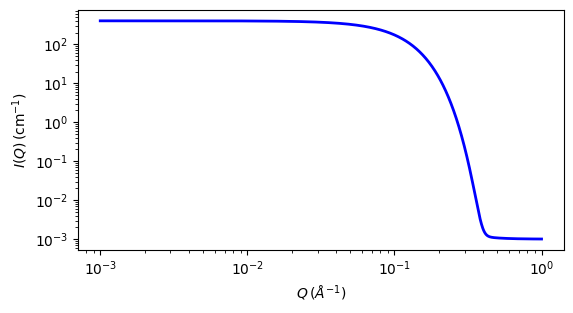
Fig. 128 1D plot corresponding to the default parameters of the model.

Source

unified_power_Rg.py

References

1. G Beaucage, J. Appl. Cryst., 28 (1995) 717-728

2. G Beaucage, J. Appl. Cryst., 29 (1996) 134-146

3. B Hammouda, Analysis of the Beaucage model, J. Appl. Cryst., (2010), 43, 1474-1478

Authorship and Verification

• Author:

• Last Modified by:

• Last Reviewed by: