Fitting

Note

If some code blocks are not readable, expand the documentation window

Preparing to fit data

To fit some data you must first load some data, activate one or more data sets, send those data sets to fitting, and select a model to fit to each data set.

Instructions on how to load and activate data are in the section Loading Data.

SasView can fit data in one of three ways:

• in Single fit mode - individual data sets are fitted independently one-by-one

• in Simultaneous fit mode - multiple data sets are fitted simultaneously to the same model with/without constrained parameters (this might be useful, for example, if you have measured the same sample at different contrasts)

• in Batch fit mode - multiple data sets are fitted sequentially to the same model (this might be useful, for example, if you have performed a kinetic or time-resolved experiment and have lots of data sets!)

Selecting a model

The models in SasView are grouped into categories. By default these consist of:

• Cylinder - cylindrical shapes (disc, right cylinder, cylinder with end-caps etc)

• Ellipsoid - ellipsoidal shapes (oblate, prolate, core shell, etc)

• Parallelepiped - as the name implies

• Sphere - spheroidal shapes (sphere, core multishell, vesicle, etc)

• Lamellae - lamellar shapes (lamellar, core shell lamellar, stacked lamellar, etc)

• Shape-Independent - models describing structure in terms of density correlation functions, fractals, peaks, power laws, etc

• Paracrystal - semi ordered structures (bcc, fcc, etc)

• Structure Factor - S(Q) models

• Plugin Models - User-created (custom/non-library) Python models

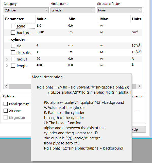
Use the Category drop-down menu to chose a category of model, then select a model from the drop-down menu to the right. The “Show Plot” button on the bottom of the dialog will become active. If you click on it, a graph of the chosen model, calculated using default parameter values, will appear. The graph will update dynamically as the parameter values are changed.

You can decide your own model categorizations using the Category Manager.

Once you have selected a model you can read its help documentation by clicking on the Help button. Additionally, right clicking on the empty space in the parameter table will display a short description of the model.

Interaction Models

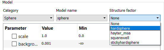
Structure factor S(Q) models can be combined with many form factor P(Q) models in the other categories to generate what SasView calls “interaction models” (previously “product models”). The combination can be done by one of two methods, but how they behave is slightly different.

The first, most straightforward, method is simply to use the S(Q) drop-down in the FitPage:

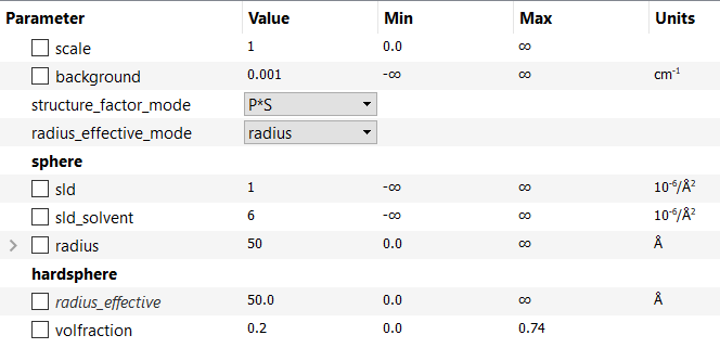
This example would then generate an interaction model with the following parameters:

The other method is to use the Add / Multiply Models tool under Fitting menu:

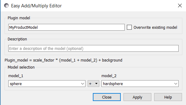
This creates an interaction model with the following parameters:

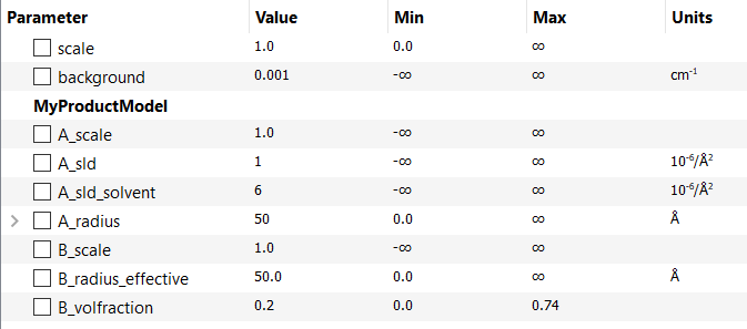
As can be seen, the second method has produced an interaction model with an extra parameter: radius_effective. This is the radial distance determining the range of the \(S(Q)\) interaction and may, or may not, be the same as the radius, in this example, depending on the concentration of the system. In other systems, radius_effective may depend on the particle form (shape). SasView offers the flexibility to automatically constrain (tie) some of these parameters together so that, for example, radius_effective = radius. See Add / Multiply Models.

Also see Fitting Models with Structure Factors for further information.

Note

SasView v5.0.4 incorporated a technical change to how the volume normalisation is incorporated in the interaction calculator that computes \(I(Q)\) from \(P(Q) S(Q)\). The change will affect all future versions of SasView. For more details, please see the Release Notes.

Mixture Models

SasView “mixture models” (previously called “sum models”) are summations of form factor models, or even of form factor models and an “interaction model” (see above), and are used to describe mixed-phase systems where the scattering is proportional to the volume fraction of each contributing phase.

Show 1D/2D

Models are normally fitted to 1D (ie, I(Q) vs Q) data sets, but some models in SasView can also be fitted to 2D (ie, I(Qx,Qy) vs Qx vs Qy) data sets.

NB: Magnetic scattering can only be fitted in SasView in 2D.

To activate 2D fitting mode, select the 2D view checkbox on the Fit Page. To return to 1D fitting model, de-select the same checkbox.

Category Manager

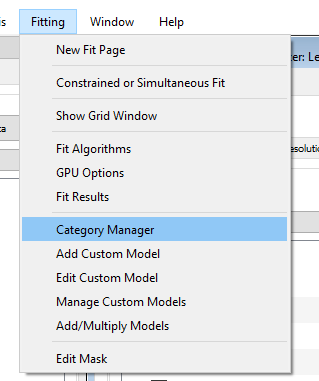
To change the model categorizations, either choose Category Manager from the View option on the menu bar, or click on the Modify button on the Fit Page.

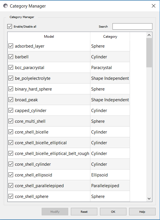
The categorization of all models except the user supplied Plugin Models can be reassigned, added to, and removed using Category Manager. Models can also be hidden from view in the drop-down menus.

Changing category

To change category, highlight a model in the list by left-clicking on its entry and then click the Modify button. Use the Change Category panel that appears to make the required changes.

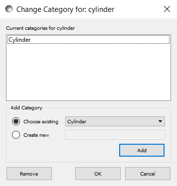
To create a category for the selected model, click the Add button. In order to delete a category, select the category name and click the Remove button. Then click OK.

Showing/hiding models

Use the Enable / Disable All buttons and the check boxes beside each model to select the models to show/hide. To apply the selection, click OK.

Model Functions

For a complete list of all the library models available in SasView, see the Model Documentation .

It is also possible to add your own models.

Adding your own Models

There are essentially four ways to generate new fitting models for SasView:

• Using the SasView Add / Multiply Models dialog to sum/multiply together two existing models in the model library (best for beginners - provided the required models are in the model library!)

• Using the SasView Add Custom Model helper dialog (aimed at those with little programming experience but works best for relatively simple models)

• By copying/editing an existing model (this can include models generated by the New Plugin Model dialog) in the Python Shell-Editor Tool or Model Editor (suitable for all use cases)

• By writing a model from scratch outside of SasView (only recommended for experienced Python users)

In the last two cases, please read the guidance on Writing a Plugin Model before proceeding.

For your model to be found by SasView it must reside in the *~\.sasview\plugin_models* folder.

Plugin Model Operations

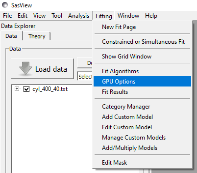
From the Fitting option in the menu bar, select one of the options:

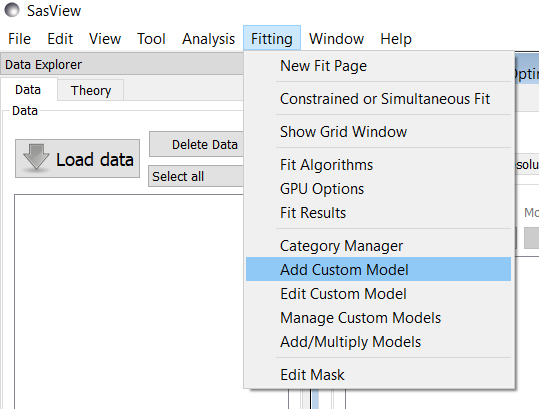
• Add Custom Model - to create a plugin model template with a helper dialog

• Edit Custom Model - to edit a plugin model in an editor window

• Manage Custom Models - to list available plugin models, add one you have written, duplicate a model, edit a model, or delete a model

• Add/Multiply Models - to create a plugin model by summing/multiplying two existing models in the model library

Add Custom Model

Relatively straightforward models can be programmed directly from the SasView GUI using the Plugin Definition Function.

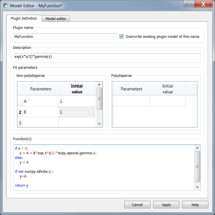
When using this feature, be aware that even if your code has errors, including syntax errors, a model file is still generated. When you then correct the errors and click ‘Apply’ again to re-compile you will get an error informing you that the model already exists if the ‘Overwrite’ box is not checked. In this case you will need to supply a new model function name. By default the ‘Overwrite’ box is checked.

Also note that the ‘Fit Parameters’ have been split into two sections: those which can be polydisperse (shape and orientation parameters) and those which are not (eg, scattering length densities).

A model file generated by this option can be viewed and further modified using the Model Editor.

It possible to specify whether a plugin created with the New Plugin Model dialog is actually a form factor P(Q) or a structure factor S(Q). To do this, simply add one or other of the following lines under the import statements.

For a form factor:

form_factor = True

or for a structure factor:

structure_factor = True

If the plugin is a structure factor it is also necessary to add two variables to the parameter list:

parameters = [
                ['radius_effective', '', 1, [0.0, numpy.inf], 'volume', ''],
                ['volfraction', '', 1, [0.0, 1.0], '', ''],
                [...],

and to the declarations of the functions Iq and Iqxy::

def Iq(x , radius_effective, volfraction, ...):

def Iqxy(x, y, radius_effective, volfraction, ...):

Such a plugin should then be available in the S(Q) drop-down box on a FitPage (once a P(Q) model has been selected).

Add / Multiply Models

Choosing the Add/Multiply models item from the Fitting menu

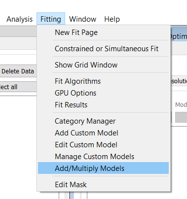
displays the Easy Add/Multiply Editor dialog.

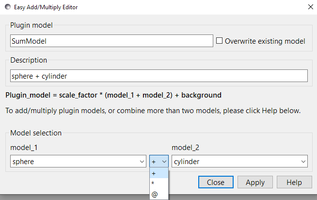
This editor allows the creation of combined custom Plugin Models. Give the new model a name (which will appear in the list of plugin models on the FitPage) and brief description (to appear under the Details button on the FitPage). The model name must not contain spaces (use underscores to separate words if necessary) and if it is longer than ~25 characters the name will not display in full in the list of models. Now select two models, as model_1 (or p1) and model_2 (or p2), and the required operator, ‘+’, ‘*’, or ‘@’ between them. Finally, click the Apply button to generate and test the model.

The + operator sums the individual I(Q) calculations and introduces a third scale factor:

Plugin Model = scale_factor * {(scale_1 * model_1) +/- (scale_2 * model_2)} + background

the * operator multiplies the individual I(Q) calculations:

Plugin Model = scale_factor * (model1 * model2) + background

and the @ operator treats the combination as a form factor [F(Q)] for model_1 and a structure factor [S(Q)] for model_2. The scale and background for F(Q) and S(Q) are set to 1 and 0 respectively and the combined model should support the beta approximation:

Plugin Model = scale_factor * vol_fraction * <FF> * S(Q) + background :: No beta
Plugin Model = scale_factor * (vol_fraction / form_volume) * (<FF> + <F>^2 * (S(Q) - 1)) + background :: beta

All Versions Changes made to a plugin model are not applied to models actively in use on fit pages. To apply plugin model changes, re-select the model from the drop-down menu on the FitPage.

In SasView 6.x, multiplicity models cannot be combined. If a model with any layer or conditional parameter is selected, similar models are removed from the other combo box.

In SasView 4.x, if the model is not listed on a fit page you can try and force a recompilation of the plugins by selecting Fitting > Plugin Model Operations > Load Plugin Models. In SasView 5.0.2 and earlier, you may need to restart the program. In SasView 5.0.3 and later, the new model should appear in the list as soon as the model is saved.

Warning

SasView versions 4.2.x, 5.0.0 and 5.0.1 The Easy Add/Multiply Editor dialog should not be used to combine a plugin model with a built-in model, or to combine two plugin models. The operation will appear to work in 4.2.x but may generate a faulty plugin model. In 5.0.0 the operation will fail (generating an error message in the Log Explorer). Whilst in 5.0.1 the operation has been blocked.

If you need to generate a plugin model from more than two built-in models, please read the sub-sections Model Structure and Combining more than two models below.

Model Structure

SasView version 4.2 introduced a much simplified and more extensible structure for plugin models generated through the Easy Sum/Multi Editor. For example, the code for a combination of a sphere model with a power law model now looks like this:

from sasmodels.core import load_model_info
from sasmodels.sasview_model import make_model_from_info

model_info = load_model_info('sphere+power_law')
model_info.name = 'MyPluginModel'
model_info.description = 'sphere + power_law'
Model = make_model_from_info(model_info)

To change the models or operators contributing to this plugin it is only necessary to edit the string in the brackets after load_model_info, though it would also be a good idea to update the model name and description too!!!

The model specification string can handle multiple models and combinations of operators (‘+’ or ‘*’) which are processed according to normal conventions. Thus ‘model1+model2*model3’ would be valid and would multiply model2 by model3 before adding model1. In this example, parameters in the FitPage would be prefixed A (for model2), B (for model3) and C (for model1). Whilst this might appear a little confusing, unless you were creating a plugin model from multiple instances of the same model the parameter assignments ought to be obvious when you load the plugin.

This streamlined approach to building complex plugin models from existing library models, or models available on the Model Marketplace, also permits the creation of P(Q)*S(Q) plugin models, something that was not possible in earlier versions of SasView. Also see Interaction Models above.

Note

Interaction Models

When the Easy Sum/Multi Editor creates a P(Q)*S(Q) model it will use the * symbol like this:

sphere*hardsphere

However, it is probably advisable to edit the model file and use the @ symbol instead, for example:

sphere@hardsphere

This is because * and @ confer different behavior on the model

• with @ - the radius and volume fraction in the S(Q) model are constrained to have the same values as the radius and volume fraction in the P(Q) model.

• with * - the radii and volume fractions in the P(Q) and S(Q) models are unconstrained.

Warning

If combining P(Q) models with S(Q) models, particularly if combining multiple instances of such models (eg, \((P(Q)_1\) * \(S(Q)_1\)) + \((P(Q)_2\) * \(S(Q)_2)\) or similar), pay careful attention to the behaviour of the scale and volume fraction parameters and test your model thoroughly, preferably on well-characterised data.

Combining more than two models

If you need generate a plugin model from more than two other models, it is tempting to think that the way to do so is simply to use the Easy Add/Multiply Editor dialog to combine the first two models into a plugin, then generate a new plugin using that first plugin as one of the selected models, combine it with the third model, and repeat as required.

This does not currently work properly (although it may appear to in SasView 4.2.x).

Instead, use the Easy Add/Multiply Editor dialog to combine the first two models, then navigate to the plugin folder (~\.sasview\plugin_models on Windows) and open the plugin Python file (eg, MyPluginModel.py) in a text editor.

Now edit the Python to specify all the models to contribute to the expanded plugin (the text string in the brackets after load_model_info). Make sure you specify the model names correctly, including any capitalisation (if in doubt use the model name dropdown on a FitPage)! Finally, update the model name and description, and save the file.

So, as an example, one could take the MyPluginModel example in the preceding section, change it to:

from sasmodels.core import load_model_info
from sasmodels.sasview_model import make_model_from_info

model_info = load_model_info('power_law+fractal+gaussian_peak+gaussian_peak')
model_info.name = 'MyBigPluginModel'
model_info.description = 'For fitting pores in crystalline framework'
Model = make_model_from_info(model_info)

and re-save it as MyBigPluginModel.py. When loaded into a FitPage, the parameters for the four models in the load_model_info string are then all present and prefixed by A_, B_, C_, and D_, respectively.

Model Editor

Selecting “Edit Custom Model” option opens the editor window.

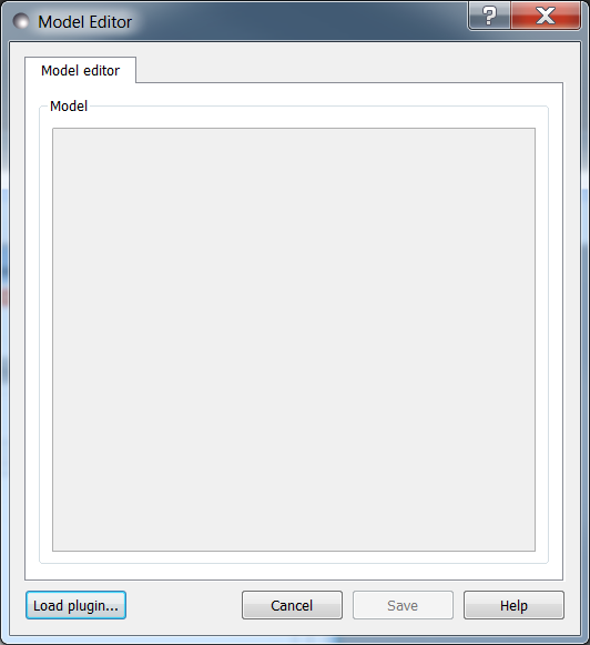
Initially, the editor is empty. A custom model can be loaded by clicking on the Load plugin… button and choosing one of the existing custom plugins.

Once the model is loaded, it can be edited and saved with Save button. Saving the model will perform the validation and only when the model is correct it will be saved to a file. Successful model check is indicated by a SasView status bar message.

When Cancel is clicked, any changes to the model are discarded and the window is closed.

For details of the SasView plugin model format see Writing a Plugin Model .

To use the model, go to the relevant Fit Page, select the Plugin Models category and then select the model from the drop-down menu.

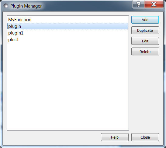
Plugin Manager

Selecting the Manage Custom Models option shows a list of all the plugin models in the plugin model folder, on Windows this is

C:\Users\{username}\.sasview\plugin_models

You can add, edit, duplicate and delete these models using buttons on the right side of the list.

Add a model

Clicking the “Add” button opens the Model Editor window, allowing you to create a new plugin as described above.

Duplicate a model

Clicking the “Duplicate” button will create a copy of the selected model(s). Naming of the duplicate follows the standard, with an n added to the plugin model name, where n is the first unused integer.

Edit a model

When a single model is selected, clicking this button will open the Advanced Model Editor allowing you to edit the Python code of the model. If no models or multiple models are selected, the Edit button is disabled.

Delete Plugin Models

Simply highlight the plugin model(s) to be removed and click on the “Delete” button. The operation is final.

NB: Models shipped with SasView cannot be removed in this way.

Fit Algorithms

It is possible to specify which optimiser SasView should use to fit the data, and to modify some of the configurational parameters for each optimiser.

From Fitting in the menu bar select Fit Algorithms, then select one of the following optimisers:

• DREAM

• Levenberg-Marquardt

• Quasi-Newton BFGS

• Differential Evolution

• Nelder-Mead Simplex

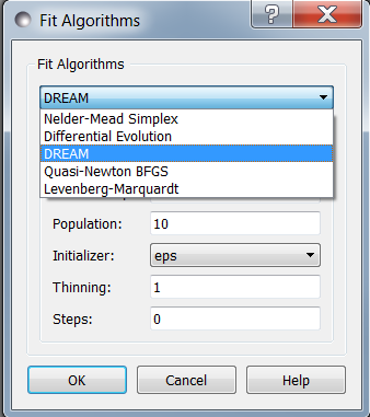
The DREAM optimiser is the most sophisticated, but may not necessarily be the best option for fitting simple models. If uncertain, try the Levenberg-Marquardt optimiser initially.

These optimisers form the Bumps package written by P Kienzle. For more information on each optimiser, see the Fitting Documentation.

Fitting Limits

By default, SasView will attempt to model fit the full range of the data; ie, across all Q values. If necessary, however, it is possible to specify only a sub-region of the data for fitting.

In a FitPage or BatchPage change the tab to Fit Options and then change the Q values in the Min and/or Max text boxes.

To return to including all data in the fit, click the Reset button.

Shortcuts

Copy/Paste Parameters

It is possible to copy the parameters from one Fit Page and to paste them into another Fit Page using the same model.

To copy parameters, either:

• Select Edit -> Copy Params from the menu bar, or

• Use Ctrl(Cmd on Mac) + Left Mouse Click on the Fit Page.

To paste parameters, either:

• Select Edit -> Paste Params from the menu bar, or

• Use Ctrl(Cmd on Mac) + Shift + Left-click on the Fit Page.

If either operation is successful a message will appear in the info line at the bottom of the SasView window.

Bookmark

To Bookmark a Fit Page either:

• Select a Fit Page and then click on Bookmark in the tool bar, or

• Right-click and select the Bookmark in the popup menu.

Status Bar & Log Explorer

The status bar is located at the bottom of the SasView window and displays messages, warnings and errors.

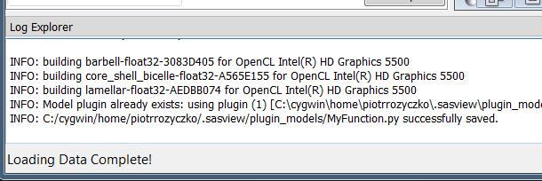
The bottom part of the SasView application window contains the Log Explorer. The Log Explorer displays available message history and run-time traceback information.

Single Fit Mode

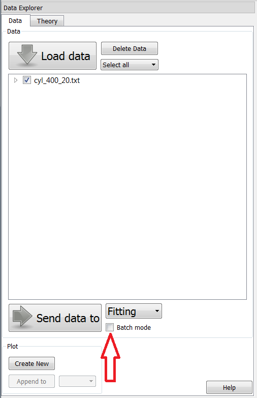
NB: Before proceeding, ensure that the Batch mode checkbox at the bottom of the Data Explorer is unchecked (see the section Loading Data ).

This mode fits one data set.

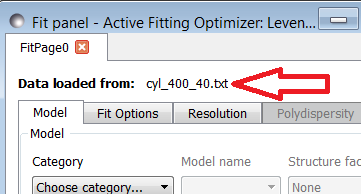
When data is sent to the fitting, the Fit Page will show the dataset name.

Clicking on the Show Plot will cause the data can be plotted in a graph window as markers.

If a graph does not appear, or a graph window appears but is empty, then the data has not loaded correctly. Check to see if there is a message in the Status Bar & Log Explorer or in the Console window.

Assuming the data has loaded correctly, when a model is selected a blue model calculation (or what SasView calls a ‘Theory’) line will appear in the earlier graph window, and a second graph window will appear displaying the residuals (the difference between the experimental data and the theory) at the same X-data values. See Assessing Fit Quality.

The objective of model-fitting is to find a physically-plausible model, and set of model parameters, that generate a theory that reproduces the experimental data and gives residual values as close to zero as possible.

Change the default values of the model parameters by hand until the theory line starts to represent the experimental data. Then uncheck the tick boxes alongside all parameters except the ‘background’ and the ‘scale’. Click the Fit button. SasView will optimise the values of the ‘background’ and ‘scale’ and also display the corresponding uncertainties on the optimised values.

NB: If no uncertainty is shown it generally means that the model is not very dependent on the corresponding parameter (or that one or more parameters are ‘correlated’).

In the bottom right corner of the Fit Page is a box displaying the normalised value of the statistical \(\chi^2\) parameter returned by the optimiser.

Now check the box for another model parameter and click Fit again. Repeat this process until most or all parameters are checked and have been optimised. As the fit of the theory to the experimental data improves the value of ‘chi2/Npts’ will decrease. A good model fit should easily produce values of ‘chi2/Npts’ that are close to one, and certainly <100. See Assessing Fit Quality.

SasView has a number of different optimisers (see the section Fit Algorithms). The DREAM optimiser is the most sophisticated, but may not necessarily be the best option for fitting simple models. If uncertain, try the Levenberg-Marquardt optimiser initially.

Polydisperse Parameters

Some model parameters, for example, radii/lengths or orientation angles can be polydisperse; i.e. they can have a distribution of possible values. Polydisperse parameters are defined as such when the model is coded, and can be activated by clicking the Polydispersity checkbox on the Fit Page.

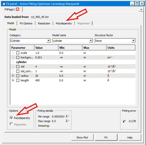
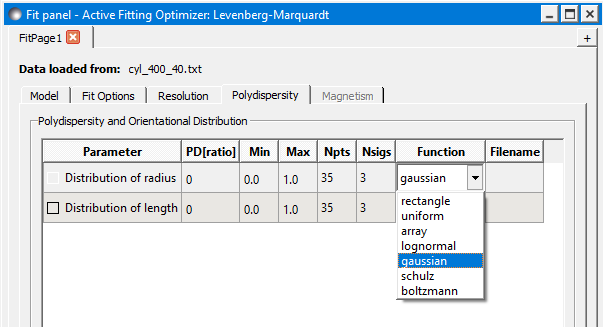
Clicking on the Polydispersity tab then provides access to these polydisperse parameters and allows the type (i.e. the function to be used) and ‘width’ (the PD[ratio]) to be adjusted. If necessary the ‘step size’ (Npts) and ‘range’ (Nsigs) of the function can also be adjusted.

For more information, see the descriptions of Polydispersity & Orientational Distributions. In particular, pay attention to the Suggested Applications and Usage Notes therein. The detail of how SasView computes the scattering from polydisperse systems is described in the Theory section.

Note that SasView defaults to Gaussian distributions, but these will not always be the best choice. Also, the definitions of the centre (e.g. whether it is the mean or median value, for example) and the actual width of the function will vary depending on the chosen distribution! For orientation distributions the PD[ratio] parameter is absolute. But for distributions applied to ‘volume’ (size) parameters the PD[ratio] parameter will always be relative to the current centre value.

Note

Polydispersity distributions in SasView define the number density of the given population of scatterers. The resulting scattering is then the number average over the distribution.

It is possible to optimise a PD[ratio] parameter during fitting by checking the accompanying checkbox. However, this is usually only effective in the latter stages of a converging fit.

Note

Neither the PD[ratio], or the parameter to which it is applied, can be optimised if using an Array Distribution. See Polydispersity & Orientational Distributions.

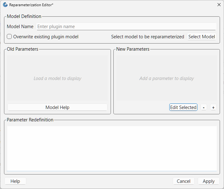
Reparameterizing Models

It is also possible to reparameterize a particle model, for instance, to give greater control over polydispersity due to intra-particle constraints, see Reparameterized Models. For example, if the particles aspect ratio is constrained but not its volume, or if its volume must be preserved but a range of aspect ratios are permitted for each volume. This may require a User-Defined distribution function to fully describe the model (see Polydispersity & Orientational Distributions).

Using a GPU

Incoporating polydispersity in a fit can certainly improve the overall solution and add a dose of realism to it (few real systems are monodisperse!). But doing so will slow the fitting process, sometimes quite dramatically. In these circumstances enabling a GPU, if present, will help.

If a potential GPU device is present the dialog will show it. The Test button can then be used to check if your system has the necessary drivers to use it. But also see GPU Setup .

Simultaneous Fit Mode

NB: Before proceeding, ensure that the Batch Mode check button at the bottom of the Data Explorer is unchecked (see the section Loading Data ).

This mode is an extension of the Single Fit Mode that fits two or more data sets to the same model simultaneously. If necessary it is possible to constrain fit parameters between data sets (eg, to fix a background level, or radius, etc).

If the data to be fit are in multiple files, load each file, then select each file in the Data Explorer, and Send To Fitting. If multiple data sets are in one file, load that file, Unselect All Data, select just those data sets to be fitted, and Send To Fitting. Either way, the result should be that for n data sets you have 2n graphs (n of the data and model fit, and n of the resulting residuals). But it may be helpful to minimise the residuals plots for clarity. Also see Assessing Fit Quality.

NB: If you need to use a custom Plugin Model, you must ensure that model is available first (see Adding your own Models ).

Method

Now go to each FitPage in turn and:

• Select the required category and model;

• Unselect all the model parameters;

• Enter some starting guesses for the parameters;

• Enter any parameter limits (recommended);

• Select which parameters will refine (selecting all is generally a bad idea…);

When done, select Constrained or Simultaneous Fit under Fitting in the menu bar.

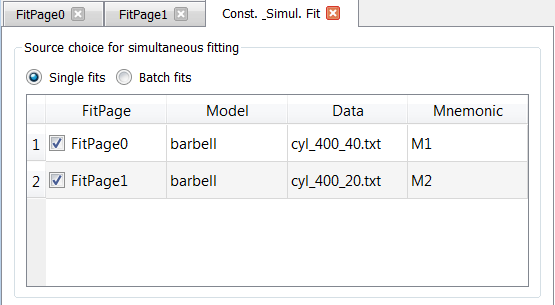
In the Const & Simul Fit page that appears, select which data sets are to be simultaneously fitted (this will probably be all of them or you would not have loaded them in the first place!).

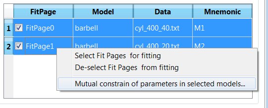
To tie parameters between the data sets with constraints, select the data sets and right click. From the menu choose Mutual constraint of parameters in selected models

When ready, click the Fit button on the Const & Simul Fit page, NOT the Fit button on the individual FitPage’s.

Simultaneous Fits without Constraints

The results of the model-fitting will be returned to each of the individual FitPage’s. Also see Assessing Fit Quality.

Simultaneous Fits with Constraints

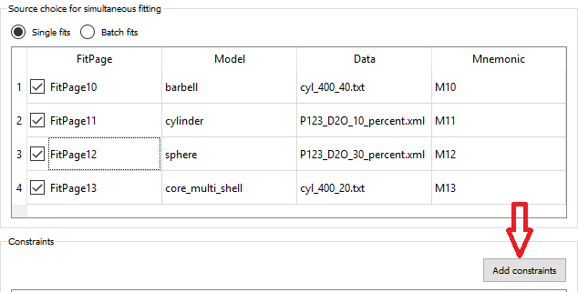
In the Const. & Simul. Fit page make sure that at least two fitpages are present. Then, click the Add constraints button

Alternatively, right clicking on two selected fitpages in the Source choice for simultaneous fitting area will bring up the context menu:

Here you can choose datasets for fitting and define constraints between parameters in both datasets.

Clicking the Add constraints button or choosing the Mutual constraint of parameters in selected models… option will bring up the Complex Constraint dialog.

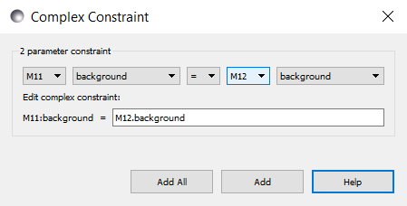
Constraints will generally be of the form

Mi:Parameter1 = Mj.Parameter1

however the text box after the ‘=’ sign can be used to adjust this relationship; for example

Mi:Parameter1 = scalar * Mj.Parameter1

A ‘free-form’ constraint box is also provided.

Many constraints can be entered for a single fit.

The results of the model-fitting will be returned to each of the individual FitPage’s. Also see Assessing Fit Quality.

Simultaneous Fits with a Modified Weighting

When simultaneously fitting different data sets, the degree of influence that each of them has on the final fit is defined by their statistical weight, i.e. mainly the number of points and their uncertainty in each data set. The SasView fitting engine tries to minimize the total \(\chi^2\), where the difference between the data and the model for each data point is added quadratically using a weight that by default is inversely proportional to the y axis error. As a consequence, datasets with more points and smaller errors will exert a greater influence on the fit. While the weighting scheme can be modified in the Fit Options tab, even setting the weighting to None (i.e. all data points from all data sets have the same weight, equal to 1) will not solve the potential issue of having disparate number of data points in different sets. In this case, if one data set has much more (less) points than the remaining data sets, it will have a much larger (smaller) influence in the global fit.

This is especially true for data gathered using different methods with different associated errors. For example attempting to fit SANS and SAXS data often leads to the SAXS data dominating the fit. The Modify Weighting option provides a way of getting around this issue by allowing the user to multiply the individual weights by a global factor that can be adjusted for each data set.

Checking the Modify Weighting box reveals a fifth column in the source choice dialog called Weighting. This is depicted in the screenshot below.

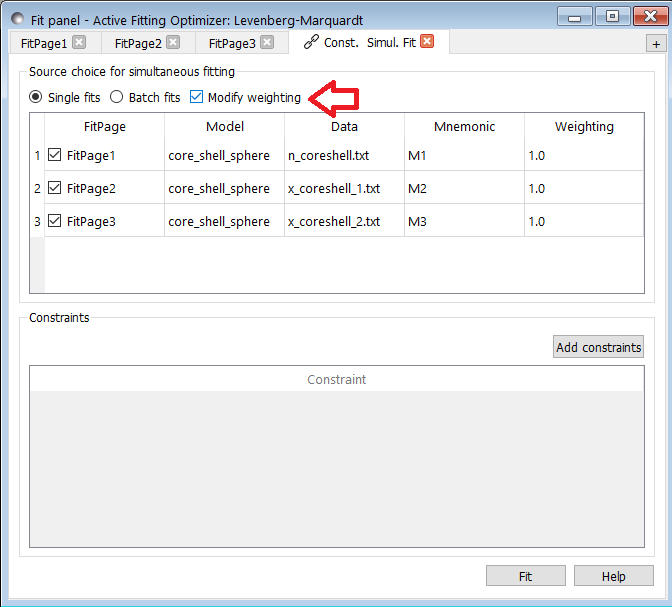
The pre-filled option in the weighting column is 1.0, and only numerical inputs (integer or floating point numbers) are allowed. It is important to understand that when the Modify Weighting box is checked, the weights of each data set will be modified, even when all the weights in the weighting column are equal to 1. Actually, when all the user weights are equal to 1, SasView will try to calculate appropriate weights in order to ensure that all the data sets have approximately a similar influence in the total fit. This is done by estimating the statistical weight of each data set j as \(W_j = \sum_i^{N_j} (1/e_i)^2\), where at present \(e_i\) is the relative error of point i, i.e. \(e_i = \sigma_i / |I_i|\), and then the weight to apply to each data set is computed as \(Min(W_j)/W_j\). Thus, the weight of the initially “lighter” set remains equal to 1, while the remaining sets will be scaled down by a factor < 1. Then the user weighting factors multiply this scaling factor, giving the final weight for each data set that will be sent to the fitting engine. The final weights used in the simultaneous fit are given in the Log Explorer window and can provide a useful indication of how much each data set has been “modified” with respect to the original data.

Warning: This option gives the user the flexibility to play with the data sets, in order to drive the global fit in a desired direction. It can be useful when a particular set contains important information to determine one or several model parameters, but it is ignored in the global fit because of statistical issues. However, ideally this option should never be needed, as difficulties when trying to fit simultaneously several sets are often an indication of other problems such as systematic errors, inadequate error/resolution estimation, etc. Therefore, users are advised to be extremely careful when using this option and to carefully check any result obtained using modified weights.

Batch Fit Mode

NB: Before proceeding, ensure that the Batch Mode check button at the bottom of the Data Explorer is unchecked (see the section Loading Data ). The Batch Mode button will be used later on!

This mode sequentially fits two or more data sets to the same model. Unlike in simultaneous fitting, in batch fitting it is not possible to constrain fit parameters between data sets.

If the data to be fit are in multiple files, load each file in the Data Explorer. If multiple data sets are in one file, load just that file. Unselect All Data, then select a single initial data set to be fitted. Fit that selected data set as described above under Single Fit Mode.

NB: If you need to use a custom Plugin Model, you must ensure that model is available first (see Adding your own Models ).

Method

Now Select All Data in the Data Explorer, check the Batch Mode check button at the bottom of that panel and Send To Fitting. A BatchPage will be created.

NB: The Batch Page can also be created by checking the Batch Mode check button and selecting New Fit Page under Fitting in the menu bar.

Using the drop-down menus in the BatchPage, now set up the same data set with the same model that you just fitted in single fit mode. A quick way to set the model parameter values is to just copy them from the earlier Single Fit. To do this, go back to the Single Fit FitPage, select Copy Params under Edit in the menu bar, then go back to the BatchPage and Paste Params.

When ready, use the Fit button on the BatchPage to perform the fitting, NOT the Fit button on the individual FitPage’s.

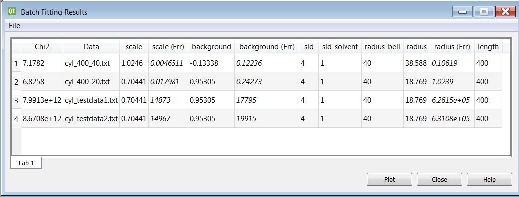
Unlike in single fit mode, the results of batch fits are not returned to the BatchPage. Instead, a spreadsheet-like Grid Window will appear.

If you want to visually check a graph of a particular fit, click on the name of a Data set in the Grid Window and then click the Plot button. The data and the model fit will be displayed.

NB: In theory, returning to the BatchPage and changing the name of the I(Q) data source should also work, but at the moment whilst this does change the data set displayed it always superimposes the ‘theory’ corresponding to the starting parameters.

Chain Fitting

By default, the same parameter values copied from the initial single fit into the BatchPage will be used as the starting parameters for all batch fits. It is, however, possible to get SasView to use the results of a fit to a preceding data set as the starting parameters for the next fit in the sequence. This variation of batch fitting is called Chain Fitting, and will considerably speed up model-fitting if you have lots of very similar data sets where a few parameters are gradually changing. Do not use chain fitting on disparate data sets.

To use chain fitting, select Chain Fitting under Fitting in the menu bar. It toggles on/off, so selecting it again will switch back to normal batch fitting.

To choose the order of the fitpages in the fitting process, drag and drop rows in the Source choice for simultaneous fitting table. The order of the table determines the order of the chain fitting performed.

Grid Window

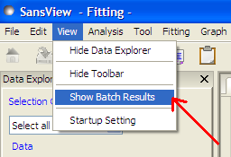
The Grid Window provides an easy way to view the results from batch fitting. It will be displayed automatically when a batch fit completes, but may be opened at any time by selecting Show Grid Window under View in the menu bar.

If there is an existing Grid Window and another batch fit is performed,* an additional ‘Table’ tab will be added to the Grid Window.

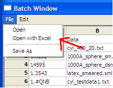
The parameter values in the currently selected table of the Grid Window can be output to a CSV file by choosing Save As under File in the (Grid Window) menu bar. The default filename includes the date and time that the batch fit was performed.

Saved CSV files can be reloaded by choosing Open under File in the Grid Window menu bar. The loaded parameters will appear in a new table tab.

NB: Saving the Grid Window does not save any experimental data, residuals or actual model fits. Consequently if you reload a saved CSV file the ability to View Fits will be lost.

Parameter Plots

Any row (dataset) can be plotted by selecting it and either right-clicking and choosing Plot selected fits menu item or by clicking on the Plot button.

Combined Batch Fit Mode

The purpose of the Combined Batch Fit is to allow running two or more batch fits in sequence without overwriting the output table of results. This may be of interest for example if one is fitting a series of data sets where there is a shape change occurring in the series that requires changing the model part way through the series; for example a sphere to rod transition. Indeed the regular batch mode does not allow for multiple models and requires all the files in the series to be fit with single model and set of parameters. While it is of course possible to just run part of the series as a batch fit using model one followed by running another batch fit on the rest of the series with model two (and/or model three etc), doing so will overwrite the table of outputs from the previous batch fit(s). This may not be desirable if one is interested in comparing the parameters: for example the sphere radius of set one and the cylinder radius of set two.

Method

In order to use the Combined Batch Fit, first load all the data needed as described in Loading Data. Next start up two or more BatchPage fits following the instructions in Batch Fit Mode but DO NOT PRESS FIT.

When done, select Constrained or Simultaneous Fit under Fitting in the menu bar.

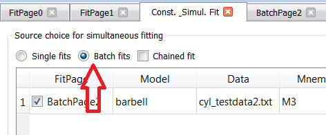
In the Const & Simul Fit page that appears, choose Batch fits radio button and select which data sets are to be fitted.

Once all are selected, click the Fit button on the Const. Simult. Fitting to run each batch fit in sequence

The batch table will then pop up at the end as for the case of the simple Batch Fitting with the following caveats:

Note

The order matters. The parameters in the table will be taken from the model used in the first BatchPage of the list. Any parameters from the second and later BatchPage s that have the same name as a parameter in the first will show up allowing for plotting of that parameter across the models. The other parameters will not be available in the grid. To choose the order of the fitpages in the fitting process, drag and drop rows in the Source choice for simultaneous fitting table.

Note

a corollary of the above is that currently models created as a sum|multiply model will not work as desired because the generated model parameters have a p#_ appended to the beginning and thus radius and p1_radius will not be recognized as the same parameter.

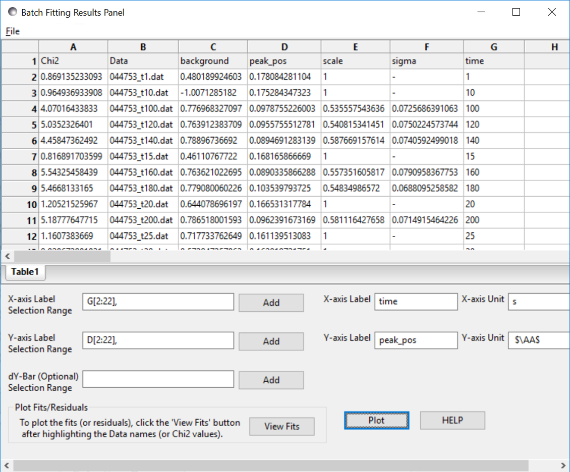
In the example shown above the data is a time series with a shifting peak. The first part of the series was fitted using the broad_peak model, while the rest of the data were fit using the gaussian_peak model. Unfortunately the time is not listed in the file but the file name contains the information. As described in Grid Window, a column can be added manually, in this case called time, and the peak position plotted against time.

Note the discontinuity in the peak position. This reflects the fact that the Gaussian fit is a rather poor model for the data and is not actually finding the peak.

Fitting SESANS Data

Since SasView version 4.1.1 it has been possible to fit SESANS data using the same fitting perspective as used to fit SANS data. This is accomplished using an on-the-fly SANS to SESANS conversion from Q-space to real-space.

To use this functionality it is important that the SESANS data file has the extension .ses to distinguish it from Q-space data. The SESANS user community is gradually refining the structure and content of its data files. Some current examples can be found in the \example_data\sesans_data folder within the SasView installation folder. For more information about the contents of .ses files, see Data Formats.

Load the .ses file and Send to Fitting as normal.

The first true indication that the data are not SANS data comes when the data are plotted. Instead of Intensity vs Q, the data are displayed as a normalised depolarisation (P) vs spin-echo length (\({\delta}\)).

Since SESANS data normally represent much longer length scales than SANS data, it will likely be necessary to significantly increase key size parameters in a model before attempting any fitting. In the screenshot above for example, the radius of the sphere could be increased from its default value of 50 Å to 5000 Å in order to get the transform to show something more sensible.

The model parameters can then be optimised by checking them as required and clicking the Fit button as is normal.

Note that SESANS data is not subject to an incoherent background signal in the way that normal SANS data is. For this reason the background parameter in any model being used to fit SESANS data should be fixed at zero.

The procedure just described supersedes the original procedure using the command line interpreter, see Fitting SESANS Data from the Command Line.

Note

This help document was last changed by Caitlyn Wolf, 20March2024