Polarisation/Magnetic Scattering

For magnetic systems, the scattering length density (SLD = \(\beta\)) is a combination of the nuclear and magnetic SLD. For polarised neutrons, the resulting effective SLD depends on the spin state of the neutron before and after being scattered in the sample.

Models in Sasview, which define a SLD parameter, can be evaluated also as magnetic models introducing the magnetisation (vector) $mathbf{M} = M (costheta_M , sin theta_M sin phi_M, sintheta_M cos phi_M)$ and the associated magnetic SLD given by the simple relation \(\beta_M = b_H M\), where \(b_H=\dfrac{\gamma r_0}{2 \mu_B} = 2.7\) fm denotes the magnetic scattering length and \(M=\lvert \mathbf{M} \rvert\) the magnetisation magnitude, where \(\gamma = -1.913\) is the gyromagnetic ratio, \(\mu_B\) is the Bohr magneton, \(r_0\) is the classical radius of electron.

It is assumed that the magnetic SLD in each region of the model is uniformly for nuclear scattering and has one effective magnetisation orientation.

The external field \(\mathbf{H}=H \mathbf{P}\) coincides with the polarisation axis $mathbf{P}=( sintheta_P cos phi_P , sin theta_P sin phi_P, costheta_P)$ for the neutrons, which is the quantisation axis for the Pauli spin operator.

Note

The polarisation axis at the sample position determines the scattering geometry. The polarisation turns adiabatically to the guide field of the instrument, before and after the field at the sample position. This operation does not change the observed spin-resolved scattering at the detector. The magnetic field defines (for random anisotropy systems) a symmetry axis and the magnetisation vector will be oriented symmetrically around the field. For AC oscillating/rotation field varying in space and with time, you can couple the magnetisation with the field axis via a constrained fit. This will allow to easily parametrise a phase shift of the magnetisation lagging behind a magnetic field varying from time frame to time frame.

The neutrons are polarised parallel (+) or antiparallel (-) to \(\mathbf{P}\). One can distinguish 4 spin-resolved cross sections:

• Non-spin-flip (NSF) \((+ +)\) and \((- -)\)

• Spin-flip (SF) \((+ -)\) and \((- +)\)

The spin-dependent magnetic scattering length densities are defined as (see Moon, Riste, and Koehler, 1969 [1])

\[\beta_{M, s_{in} s_{out}} = b_H\sigma \cdot \mathbf{M}_{\perp}\]

where \(\sigma\) is the Pauli spin, and \(s_{in/out}\) describes the spin state of the neutron before and after the sample.

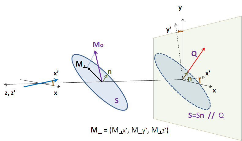
For magnetic neutron scattering, only the magnetisation component or Halpern-Johnson vector \(\mathbf{M}_{\perp}\) perpendicular to the scattering vector \(\mathbf{Q}= \hat{\mathbf{q}}=\hat{\mathbf{q}} (\cos\theta, \sin \theta,0)\) contributes to the magnetic scattering:

\[\mathbf{M}_{\perp} = \hat{\mathbf{q}} [\hat{\mathbf{q}} \cdot \mathbf{M}] - \mathbf{M}\]

with \(\hat{\mathbf{q}}\) the unit scattering vector and \(\theta\) denotes the angle between \(\mathbf{Q}\) and the x-axis.

The two NSF cross sections are given by

\[I^{\pm\pm} = N^2 \mp \mathbf{P}\cdot(N^{\ast}\mathbf{M}_{\perp} + N\mathbf{M}_{\perp}^{\ast}) + (\mathbf{P}\cdot \mathbf{M}_{\perp})^2\]

and the two SF channels:

\[I^{\pm\mp} = \mathbf{M}_{\perp}\cdot \mathbf{M}_{\perp} - (\mathbf{P}\cdot \mathbf{M}_{\perp})^2 \mp i \mathbf{P}\cdot \mathbf{M}_{\perp} \times \mathbf{M}_{\perp}^{\ast}\]

with \(i=\sqrt{-1}\), and \(^{\ast}\) denoting the complex conjugate quantity, and \(\times\) and \(\cdot\) the vector and scalar product, respectively. For symmetric, collinear spin structures (\(\mathbf{M}_{\perp} = \mathbf{M}_{\perp}^{\ast}\)), and the last term vanishes.

For the NSF scattering the component of the Halpern-Johnson vector parallel to \(P\) contributes

\[\mathbf{M}_{\perp,\parallel P } = ( \mathbf{P} \cdot \mathbf{M}_{\perp}) \mathbf{P}\]

In SasView, form factor models expect a scattering length density (SLD) as parameter. For the NSF state, the effective SLD is simply

\[\rho_{\pm\pm } = \rho_N \mp b_H \mathbf{P} \cdot \mathbf{M}_{\perp}\]

The magnetic scattering vector component perpendicular to the polarisation gives rise to SF scattering

\[\mathbf{M}_{\perp,\perp P } = \mathbf{M}_{\perp } - (\mathbf{P} \cdot \mathbf{M}_{\perp }) \mathbf{P}\]

This vector can itself again be decomposed in two contributions from the base vectors spanning the plane perpendicular to \(\mathbf{P}\). This allows to construct the purely magnetic SLD for the SF state.

Every magnetic scattering cross section can be constructed from an incoherent mixture of the 4 spin-resolved spin states depending on the efficiency parameters before (\(u_i\)) and after (\(u_f\)) the sample. For a half-polarised experiment(SANSPOL with \(u_f=0.5\)) or full (longitudinal) polarisation analysis, the accessible spin states are measured independently and a simultaneous analysis of the measured states is performed, tying all the model parameters together except \(u_i\) and \(u_f\), which are set based on the (known) polarisation efficiencies of the instrument.

Note

The values of the ‘up_frac_i’ (\(u_i\)) and ‘up_frac_f’ (\(u_f\)) must be in the range 0 to 1. The parameters ‘up_frac_i’ and ‘up_frac_f’ can be easily associated to polarisation efficiencies ‘e_in/out’ (of the instrument). Efficiency values range from 0.5 (unpolarised beam) to 1 (perfect optics) or 0 (perfect optics, but other spin state). For ‘up_frac_i/f’ < 0.5 a cross section is constructed with the spin reversed/flipped with respect to the initial supermirror polariser. The actual polarisation efficiency in this case is however ‘e_in/out’ = 1 -‘up_frac_i/f’.

User Input

The following user input parameters are used:

sld_M - the magnetic scattering length density :math:`b_H M`
sld_mtheta - the polar angle :math:`\theta_M` of the magnetisation vector
sld_mphi - the azimuthal angle :math:`\phi_M` of the magnetisation vector
up_frac_i - polarisation efficiency :math:`u_i` *before* the sample
up_frac_f - polarisation efficiency :math:`u_f` *after* the sample
p_theta - the inclination :math:`\theta_P` of the polarisation from the beam axis
p_phi - the rotation angle :math:`\phi_P` around the incoming beam axis

References

[1]

R. M. Moon and T. Riste and W. C. Koehler, Phys. Rev., 181 (1969) 920.

Document History

2015-05-02 Steve King

2017-11-15 Paul Kienzle

2018-06-02 Adam Washington

2020-12-08 Dirk Honecker