Scripting Interface¶

Preparing your environment¶

You can use python scripts to load and plot your data, create SAS models and fit parameters. You can save a script to a file such as example/model.py and run it later. However, this requires a scripting environment with the correct packages installed.

You can either use the SasView application itself (versions after 5.0.5), as both bumps and sasmodels are included as part of the distribution, so for example on Windows:

> sasview model.py

(Note that it may be necessary to first add the folder path to sasmodels/sasview to your Path environment variable for this to work; set PATH=%PATH%;C:\your\path\here\ . The folder path can be found in the Help > About box if you are running the SasView GUI.)

or create a Python environment with pip:

> pip install sasmodels sasdata matplotlib bumps periodictable
> python model.py

(You can also create a Python environment using conda, see: https://github.com/SasView/sasview/wiki/DevNotes_CondaDevEnviroment)

The pip command also works within a Jupyter notebook

%pip install sasmodels sasdata matplotlib bumps periodictable

On a Mac the command for invoking SasView will be something like:

/Applications/Sasview5.dmg/Contents/MacOS/sasview

depending on where it is actually installed. This can either be used directly or can be symlinked into your path, for example:

mkdir ~/bin
ln -s /path/to/Applications/SasView5.dmg/Contents/MacOS/sasview ~/bin

Preparing your data¶

The key functions are then core.load_model() for loading the model definition and compiling the kernel and data.load_data() for calling sasview to load the data.

Usually you will load data via the sasview loader, with the data.load_data() function. For example:

from sasmodels.data import load_data
data = load_data("sasmodels/example/093191_201.dat")

You may want to apply a data mask, such a beam stop, and trim high \(q\):

from sasmodels.data import set_beam_stop
set_beam_stop(data, qmin, qmax)

The data.set_beam_stop() method simply sets the mask attribute for the data.

The data defines the resolution function and the q values to evaluate, so even if you simulating experiments prior to making measurements, you still need a data object for reference. Use data.empty_data1D() or data.empty_data2D() to create a container with a given \(q\) and \(\Delta q/q\). For example:

import numpy as np
from sasmodels.data import empty_data1D

# 120 points logarithmically spaced from 0.005 to 0.2, with dq/q = 5%
q = np.logspace(np.log10(5e-3), np.log10(2e-1), 120)
data = empty_data1D(q, resolution=0.05)

To use a more realistic model of resolution, or to load data from a file format not understood by SasView, you can use data.Data1D or data.Data2D directly. The 1D data uses x, y, dx and dy for \(x = q\) and \(y = I(q)\), and 2D data uses x, y, z, dx, dy, dz for \(x, y = qx, qy\) and \(z = I(qx, qy)\). [Note: internally, the Data2D object uses SasView conventions, qx_data, qy_data, data, dqx_data, dqy_data, and err_data.]

For USANS data, use 1D data, but set dxl and dxw attributes to indicate slit resolution:

data.dxl = 0.117

See resolution.slit_resolution() for details.

SESANS data is more complicated; if your SESANS format is not supported by SasView you need to define a number of attributes beyond x, y. For example:

SElength = np.linspace(0, 2400, 61) # [A]
data = np.ones_like(SElength)
err_data = np.ones_like(SElength)*0.03

class Source:
    wavelength = 6 # [A]
    wavelength_unit = "A"
class Sample:
    zacceptance = 0.1 # [A^-1]
    thickness = 0.2 # [cm]

class SESANSData1D:
    #q_zmax = 0.23 # [A^-1]
    lam = 0.2 # [nm]
    x = SElength
    y = data
    dy = err_data
    sample = Sample()
data = SESANSData1D()

x, y = ... # create or load sesans
data = smd.Data

The data module defines various data plotters as well.

Using sasmodels directly¶

Once you have a computational kernel and a data object, you can evaluate the model for various parameters using direct_model.DirectModel. The resulting object f will be callable as f(par=value, …), returning the \(I(q)\) for the \(q\) values in the data. For example:

import numpy as np
from sasmodels.data import empty_data1D
from sasmodels.core import load_model
from sasmodels.direct_model import DirectModel

# 120 points logarithmically spaced from 0.005 to 0.2, with dq/q = 5%
q = np.logspace(np.log10(5e-3), np.log10(2e-1), 120)
data = empty_data1D(q, resolution=0.05)
kernel = load_model("ellipsoid)
f = DirectModel(data, kernel)
Iq = f(radius_polar=100)

Polydispersity information is set with special parameter names:

par_pd for polydispersity width, \(\Delta p/p\),

par_pd_n for the number of points in the distribution,

par_pd_type for the distribution type (as a string), and

par_pd_nsigmas for the limits of the distribution.

Using sasmodels through the bumps optimizer¶

Like DirectModel, you can wrap data and a kernel in a bumps model with bumps_model.Model and create a bumps_model.Experiment that you can fit with the bumps interface. Here is an example from the example directory such as example/model.py:

import sys
from bumps.names import *
from sasmodels.core import load_model
from sasmodels.bumps_model import Model, Experiment
from sasmodels.data import load_data, set_beam_stop, set_top

""" IMPORT THE DATA USED """
radial_data = load_data('DEC07267.DAT')
set_beam_stop(radial_data, 0.00669, outer=0.025)
set_top(radial_data, -.0185)

kernel = load_model("ellipsoid")

model = Model(kernel,
    scale=0.08,
    radius_polar=15, radius_equatorial=800,
    sld=.291, sld_solvent=7.105,
    background=0,
    theta=90, phi=0,
    theta_pd=15, theta_pd_n=40, theta_pd_nsigma=3,
    radius_polar_pd=0.222296, radius_polar_pd_n=1, radius_polar_pd_nsigma=0,
    radius_equatorial_pd=.000128, radius_equatorial_pd_n=1, radius_equatorial_pd_nsigma=0,
    phi_pd=0, phi_pd_n=20, phi_pd_nsigma=3,
    )

# SET THE FITTING PARAMETERS
model.radius_polar.range(15, 1000)
model.radius_equatorial.range(15, 1000)
model.theta_pd.range(0, 360)
model.background.range(0,1000)
model.scale.range(0, 10)

#cutoff = 0     # no cutoff on polydisperisity loops
#cutoff = 1e-5  # default cutoff
cutoff = 1e-3  # low precision cutoff
M = Experiment(data=radial_data, model=model, cutoff=cutoff)
problem = FitProblem(M)

To run the model from your python environment use the installed bumps program:

>>> bumps example/model.py --preview

Alternatively, on Windows, bumps can be called from the cmd prompt as follows:

> sasview -m bumps.cli example/model.py --preview

Calling the computation kernel¶

Getting a simple function that you can call on a set of q values and return a result is not so simple. Since the time critical use case (fitting) involves calling the function over and over with identical \(q\) values, we chose to optimize the call by only transfering the \(q\) values to the GPU once at the start of the fit. We do this by creating a kernel.Kernel object from the kernel.KernelModel returned from core.load_model() using the kernel.KernelModel.make_kernel() method. What it actual does depends on whether it is running as a DLL, as OpenCL or as a pure python kernel. Once the kernel is in hand, we can then marshal a set of parameters into a details.CallDetails object and ship it to the kernel using the direct_model.call_kernel() function. To accesses the underlying \(<F(q)>\) and \(<F^2(q)>\), use direct_model.call_Fq() instead.

The following example should help, example/cylinder_eval.py:

from numpy import logspace, sqrt
from matplotlib import pyplot as plt
from sasmodels.core import load_model
from sasmodels.direct_model import call_kernel, call_Fq

model = load_model('cylinder')
q = logspace(-3, -1, 200)
kernel = model.make_kernel([q])
pars = {'radius': 200, 'radius_pd': 0.1, 'scale': 2}
Iq = call_kernel(kernel, pars)
F, Fsq, Reff, V, Vratio = call_Fq(kernel, pars)

plt.loglog(q, Iq, label='2 I(q)')
plt.loglog(q, F**2/V, label='<F(q)>^2/V')
plt.loglog(q, Fsq/V, label='<F^2(q)>/V')
plt.xlabel('q (1/A)')
plt.ylabel('I(q) (1/cm)')
plt.title('Cylinder with radius 200.')
plt.legend()
plt.show()

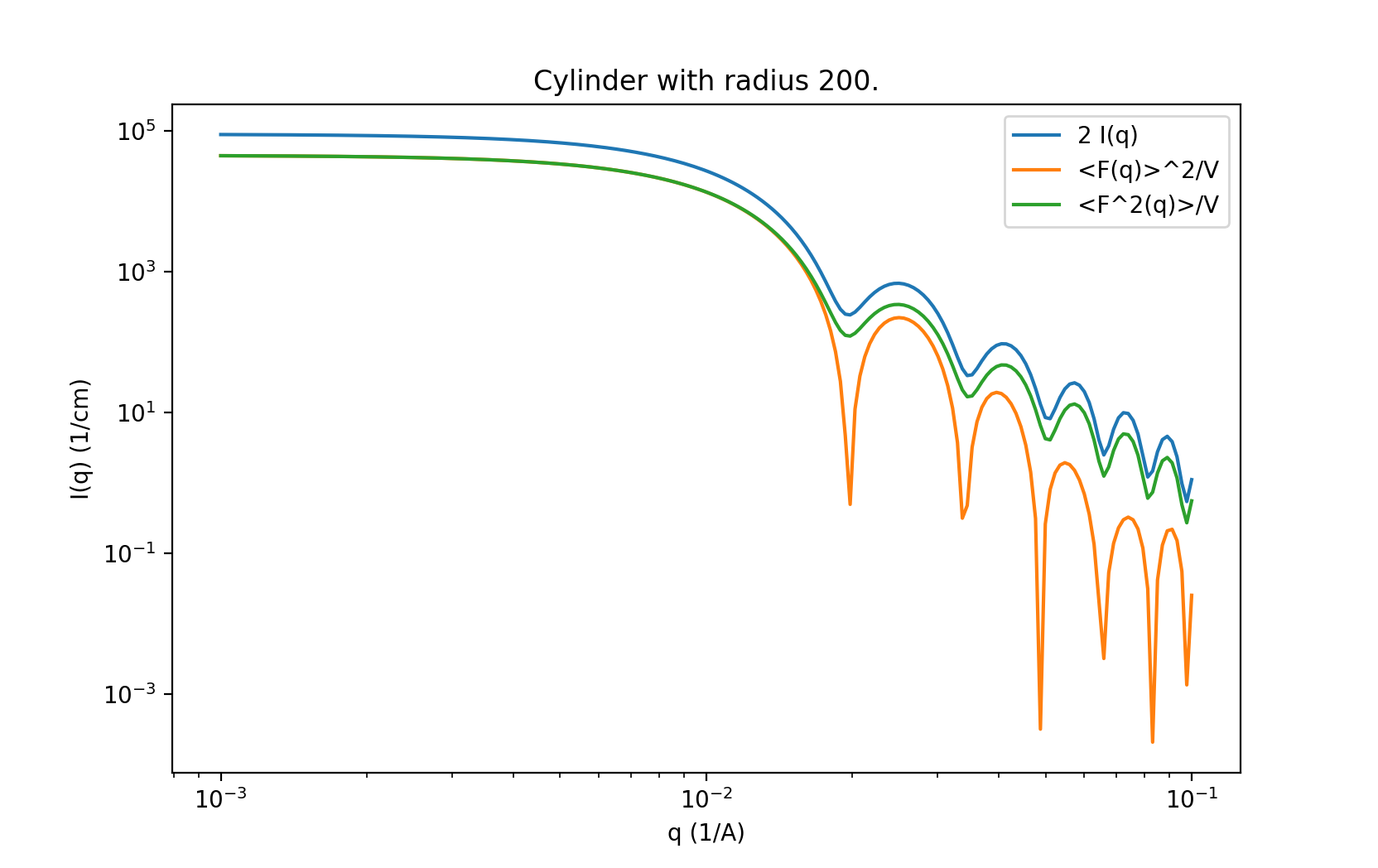
../../../../_images/direct_call.png — Fig. 144 Comparison between \(I(q)\), \(<F(q)>\) and \(<F^2(q)>\) for cylinder model.¶

This compares \(I(q)\) with \(<F(q)>\) and \(<F^2(q)>\) for a cylinder with radius=200 +/- 20 and scale=2. Note that call_Fq does not include scale and background, nor does it normalize by the average volume. The definition of \(F = \rho V \hat F\) scaled by the contrast and volume, compared to the canonical cylinder \(\hat F\), with \(\hat F(0) = 1\). Integrating over polydispersity and orientation, the returned values are \(\sum_{r,w\in N(r_o, r_o/10)} \sum_\theta w F(q,r_o,\theta)\sin\theta\) and \(\sum_{r,w\in N(r_o, r_o/10)} \sum_\theta w F^2(q,r_o,\theta)\sin\theta\).

On Windows, this example can be called from the cmd prompt using sasview as as the python interpreter:

> sasview example/cylinder_eval.py

Using sasmodels and bumps from a Jupyter notebook¶

You can also use sasmodels/bumps to fit experimental data from a Jupyter notebook by constructing and computing the model in an analogous manner to that shown above. For an example notebook see:

https://github.com/SasView/documents/blob/master/Notebooks/sasmodels_fitting.ipynb

Scripting Interface¶

Preparing your environment¶

Preparing your data¶

Using sasmodels directly¶

Using sasmodels through the bumps optimizer¶

Calling the computation kernel¶

Using sasmodels and bumps from a Jupyter notebook¶

Table of Contents

Previous topic

Next topic

This Page