Invariant Calculation

Principle

For any multi-phase system, i.e. any system that contains regions with different scattering length densities (SLD), the integral over all \(\vec{q}\) of the appropriately dimensionally-weighted scattering cross-section (ie, ‘intensity’, \(I(\vec{q})\) in absolute units) is a constant directly proportional to the mean-square average fluctuation in SLD and the phase composition. Usefully, this value is independent of the sizes, shapes, or interactions, or, more generally, the arrangement, of the phase domains (i.e. it is invariant) provided the system is incompressible (i.e, the relative volume fractions of the phases do not change). For the purposes of this discussion, a phase is any portion of the material which has a SLD that is distinctly different from the average SLD of the material. This constant is known as the Scattering Invariant, the Porod Invariant, or simply as the Invariant, \(Q^*\).

Note

In this document we shall denote the invariant by the often encountered symbol \(Q^*\). But the reader should be aware that other symbols can be encountered in the literature. Glatter & Kratky[1], and Stribeck[2], for example,both use \(Q\), the same symbol we use to denote the scattering vector in SasView(!), whilst Melnichenko[3] uses \(Z\). Other variations include \(Q_I\).

As the invariant is a fundamental law of scattering, it can be used for sanity checks (for example, scattering patterns from the same sample that may look very different should have the same invariant if the hypothesis of what is going on in the sample is correct), to cross-calibrate different SAS instruments, and, as explained below, can yield an independent estimate of volume fractions or contrast terms.

Implementation

Calculation

Assuming isotropic scattering, acquired on a typical ‘pinhole geometry’ instrument, the invariant integral can be computed from the 1D reduced data (assuming the reduced data has removed all background from sample holders,incoherent scattering in the case of neutrons, etc.) as:

\[Q^* = \int_0^\infty q^2I(q)\,dq\]

Warning

SasView, and to our knowlege most, if not all, other software implementations of this calculation, does not include the effects of instrumental resolution on the equation above. This means that for data with very significant resolution smearing (more likely to be encountered with SANS than with SAXS data) the calculated invariant will be somewhat high (though in most real cases this will probably not be the dominant uncertainty).

Note

The observant reader may notice the lack of a \(4 \pi\) prefactor in the above equation which would be required for an integral over all \(q\) stated at the beginning. This seems to be the convention historically adopted and is only important when extracting terms from the invariant as below. As long as the same convention is applied in their derivation all is consistent.

Note

Also note that if some residual flat background remains in the data, it can be corrected for if the amount can be estimated as disucussed in the usage section below.

In the extreme case of “infinite” slit smearing, the above equation reduces to:

\[Q^* = \Delta q_v \int_0^\infty qI(q)\,dq\]

where \(\Delta q_v\) is the slit height, and should be valid as long as \(\Delta q_v\) is large enough to include most, if not all, the scattering. This limit is applicable, for example, to most data taken on Bonse-Hart type instruments. SasView does implement this limit so that, in contrast to above, the invariant calculated from such slit-smeared data could be more accurate than for normal pinhole SANS data which typically has sigificant \(\Delta q / q\).

The slit smeared expression above has also been used to compute the invariant from unidirectional cuts through 2D scattering patterns such as, for example, those arising from oriented fibers (see the Crawshaw[4] and Shioya[5] references). However, in order to use the Invariant analysis window to do this, it would first be necessary to put the cuts in a data format that SasView recognises as slit-smeared by properly including the value of \(q_v\) in the data file.

Note

Currently SasView will only account for slit smearing if the data being processed by the Invariant analysis are recognized as slit smeared. It does not allow for manually inputing a slit value. Currently, only the canSAS *.XML and NIST *.ABS formats facilitate slit smeared data. The easiest way to include \(\Delta q_v\) in simple ASCII column data in a way recognizable by SasView is to mimic the *.ABS format. The data must follow the normal rules for general ASCII files but include 6 columns. The SasView general ASCII reader assumes the first four columns are \(q\), \(I(q)\), \(dI\), \(\sigma(q)\). If the data does not contain any \(dI\) information, these can be faked by making them ~1% (or less) of the \(I\) data. The fourth column must contain the \(q_v\) value, in Å^-1, but as a negative number. Each row of data should have the same value. The 5th column must be a duplicate of column 1. Column 6 can have any value but cannot be empty. Finally, the line immediately preceding the actual columnar data must begin with: “The 6 columns”. For an example, see the example data set 1umSlitSmearSphere.ABS in the \test\1d folder).

Data Extrapolation

The difficulty with using \(Q^*\) arises from the fact that experimental data is never measured over the range \(0 \le q \le \infty\) and it is thus usually necessary to extrapolate the experimental data to both low and high \(q\). Currently, SasView allows extrapolation to any user-defined low and high \(q\). The default range is \(10^{-5} \le q \le 10\) Å^-1. Note that the integrals above are weighted by \(q^2\) or \(q\). Thus the high-\(q\) extrapolation is weighted far more heavily than the low-\(q\) extrapolation so that having data measured to as large a value of \(q_{max}\) as possible can be surprisingly important.

Low-\(q\) region (<= \(q_{min}\) in data):

• The Guinier function \(I_0.exp(-q^2 R_g^2/3)\) can be used, where \(I_0\) and \(R_g\) are obtained by fitting the data within the range \(q_{min}\) to \(q_{min+j}\) where \(j\) is the user-chosen number of points from which to extrapolate. The default is the first 10 points. Alternatively a power law, similar to the high \(q\) extrapolation, can be used but this is not recommended!

High-\(q\) region (>= \(q_{max}\) in data):

• The power law function \(A/q^m\) is used where the power law constant \(m\) can be fixed to some value by the user or fit along with the constant \(A\). \(m\) will typically be between 3 and 4 for pinhole resolution with 4 indicating sharp interfaces and smaller values more diffuse interfaces. In real systems this may not always hold of course, but the user should think about what a deviation means and to what extent it is valid to use such an extrapolation. The fitted constant(s) \(A\) (\(m\)) is/are obtained by fitting the data within the range \(q_{max-j}\) to \(q_{max}\) where, again, \(j\) is the user chosen number of points from which to extrapolate, the default again being the last 10 points.

Note

While the high \(q\) exponent should generally be close to 4 for a system with sharp interfaces, in the special case of infinite slit smearing that power law should be 3 for the same sharp interfaces.

Invariant

SasView implements the invariant calculation for a two-phase (or pseudo two-phase) system, which represents the most commonly encountered situation. The invariant for this is

\[Q^* = {2 \pi^2 (\Delta\rho)^2 \phi_1 \phi_2}\]

where \(\Delta\rho = (\rho_1 - \rho_2)\) is the SLD contrast and \(\phi_1\) and \(\phi_2\) are the volume fractions of the two phases (\(\phi_1 + \phi_2 = 1\)). Thus from the invariant one can either calculate the volume fractions of the two phases given the contrast or, calculate the contrast given the volume fraction. However, the current implementation in SasView only allows for the former: extracting the volume fraction given a known contrast factor.

Volume Fraction

In some cases, especially in non-particulate systems for which no good analytical model description exists (as then the scale factor of such a model would return the volume fraction information), if the contrast term can be reasonably estimated then the invariant can provide an estimate of the volume fraction. This is quite common, for example, in the Geosciences and Materials Science where the amount of porosity in a sample (the second phase) is of vital interest.

Rearranging the above expression for \(Q^*\) yields

\[\phi_1 \phi_2 = \frac{Q^*}{2 \pi^2 (\Delta\rho)^2} \equiv A\]

and thus, if \(\phi_1 < \phi_2\)

\[\begin{split}&\phi_1 = \frac{1 - \sqrt{1 - 4A}}{2} \\ &\phi_2 = \frac{1 + \sqrt{1-4A}}{2}\end{split}\]

where \(\phi_1\) (the volume fraction of the minority phase) is reported as the the volume fraction in the Invariant analysis window.

Note

If A>0.25 then the program is obviously unable to compute \(\phi_1\). In these circumstances the Invariant window will show the volume fraction as ERROR. Possible reasons for this are that the contrast has been incorrectly entered, or that the dataset is simply not suitable for invariant analysis.

Specific Surface Area

The total surface area per unit volume is an important quantity for a variety of applications, for example, to understand the absorption capacity, reactivity, or catalytic activity of a material. This value, known as the specific surface area \(S_v\), is reflected in the scattering of the material. Indeed, any interfaces in the material separating regions of different scattering length densities contribute to the overall scattering.

For a two phase system, \(S_v\) can be computed from the scattering data as:

\[S_v = \frac{C_p}{2 \pi (\Delta\rho)^2}\]

where \(C_p\), the Porod Constant, is given by Porod’s Law:

\[Cp = \lim_{q \to \infty}I(q) q^4\]

which can be estimated from a Porod model fit to the an appropriately high-\(q\) portion of the data or from the intercept of a linear fit to the high-\(q\) portion of a Porod Plot: \(I(q)*q^4\) vs \(q^4\) (see the Porod model documentation in the Models Documentation for more details).

This calculation is unrelated to the Invariant other than to obtain the contrast term if it is not known (and the volume fraction is known), and depends only on two values - the contrast and Porod Constant - which must be provided.

Extension to Three or More Phases

In principle, as suggested in the Introduction, the invariant is a completely general concept and not limited to two phases. Extending the formalism to more phases, so that useful information can be extracted from the invariant is, however, more difficult.

We note here that in the more generalized formalism the contrast term is replaced by a quantity called the SLD fluctuation, \(\eta\), so that:

\[Q^* = {2 \pi^2 \langle \eta^2 \rangle}\]

where \(\eta\) represents the deviation in SLD from the weighted-average value, \(\langle (\rho^*) \rangle\), at any given point in the system. The mean-square average of the SLD fluctuations, \(<\eta^2>\), is:

\[\langle \eta^2 \rangle = \langle (\rho^*)^2 \rangle - \langle (\rho^*) \rangle^2\]

Returning to the simplest case of a two-phase system, this formalism can be shown to reduce to the same results given above:

\[\langle (\rho^*)^2 \rangle = \phi_1 \rho_1^2 + \phi_2 \rho_2^2\]

\[\langle (\rho^*) \rangle = \phi_1 \rho_1 + \phi_2 \rho_2\]

Setting

\[\eta_1 = \phi_2 (\rho_1 - \rho_2)\]

\[\eta_2 = \phi_1 (\rho_2 - \rho_1)\]

then yields:

\[\langle \eta^2 \rangle = \phi_1 \eta_1^2 + \phi_2 \eta_2^2 \equiv \phi_1 \phi_2 (\rho_1 - \rho_2)^2\]

and thus for the two phase system we recover:

\[Q^* = {2 \pi^2 (\Delta\rho)^2 \phi_1 \phi_2}\]

Note

For a fuller discussion of the extension of Invariant Analysis to three phases, see the Melnichenko reference[3], Chapter 6, Section 6.9, and the Shioya reference[4].

Using invariant analysis

Load some data with the Data Explorer.

Select a dataset and use the Send To button on the Data Explorer to load the dataset into the Invariant panel. Or select Invariant from the Analysis category in the menu bar.

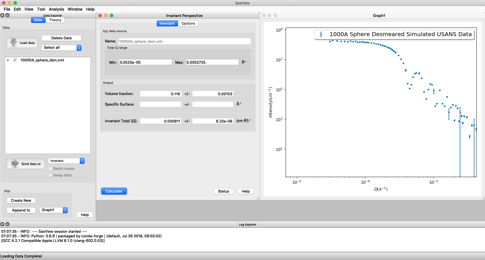
A first estimate of \(Q^*\) should be computed automatically but should be ignored as it will be incorect until the proper contrast term is specified.

Use the box on the Options tab to specify the contrast term(i.e. difference in SLDs). Note this must be specified for the eventual value of \(Q^*\) to be on an absolute scale and to therefore have any meaning).

Warning

The user must provide the correct SLD contrast for the data they are analysing in the Options tab of the Invariant window and then click on Compute before examining/using any displayed value of the invariant or volume fraction. The default contrast has been deliberately set to the unlikley-to-be-realistic value of 8e-06 Å^-2.

Optional: Also in this tab a background term to subtract from the data can be specified (if the data is not already properly background subtracted), the data can be rescaled if necessary (e.g. to be on an absolute scale) and a value for \(C_p\) can be specified (required if the specific surface area \(S_v\) is desired).

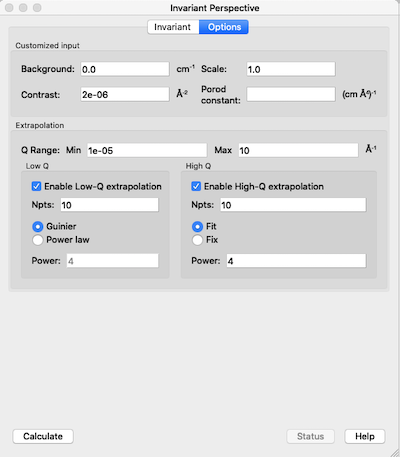
Adjust the extrapolation types as necessary by checking the relevant Enable Extrapolate check boxes. If power law extrapolations are chosen, the exponent can be either held fixed or fitted. The number of points, \(Npts\), to be used for the basis of the extrapolation can also be specified.

In most cases the default values will suffice. Click the Compute button.

Note

As mentioned above in the Data Extrapolation section, the extrapolation ranges are currently fixed and not adjustable. They are designed to keep the computation time reasonable while including as much of the total \(q\) range as should be necessary for any SAS data.

The details of the calculation are available by clicking the Status button at the bottom right of the panel.

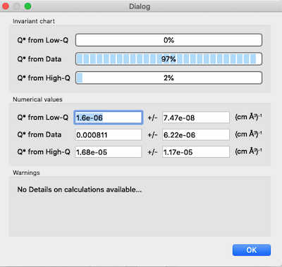
If more than 10% of the computed \(Q^*\) value comes from the areas under the extrapolated curves, proceed with caution.

References

[1]

O. Glatter and O. Kratky Chapter 2 and Chapter 14 in Small Angle X-Ray Scattering; Academic Press, New York, 1982. Available at: http://web.archive.org/web/20110824105537/http://physchem.kfunigraz.ac.at/sm/Service/Glatter_Kratky_SAXS_1982.zip.

[2]

N. Stribeck Chapter 8 in X-Ray Scattering of Soft Matter Springer, 2007.

[3] (1,2)

Y.B. Melnichenko Chapter 6 in Small-Angle Scattering from Confined and Interfacial Fluids; Springer, 2016.

[4] (1,2)

J. Crawshaw, M.E. Vickers, N.P. Briggs, R.K. Heenan, R.E. Cameron Polymer, 41 1873-1881 (2000).

[5]

13. Shioya and A. Takaku J. Appl. Phys., 58 4074 (1985).

Note

This help document was last changed (completely re-written) by Paul Butler and Steve King, March-July 2020