core_shell_parallelepiped

Rectangular solid with a core-shell structure.

Parameter	Description	Units	Default value
scale	Source intensity	None	1
background	Source background	cm-1	0.001
sld_core	Parallelepiped core scattering length density	10-6Å-2	1
sld_a	Parallelepiped A rim scattering length density	10-6Å-2	2
sld_b	Parallelepiped B rim scattering length density	10-6Å-2	4
sld_c	Parallelepiped C rim scattering length density	10-6Å-2	2
sld_solvent	Solvent scattering length density	10-6Å-2	6
length_a	Shorter side of the parallelepiped	Å	35
length_b	Second side of the parallelepiped	Å	75
length_c	Larger side of the parallelepiped	Å	400
thick_rim_a	Thickness of A rim	Å	10
thick_rim_b	Thickness of B rim	Å	10
thick_rim_c	Thickness of C rim	Å	10
theta	In plane angle	degree	0
phi	Out of plane angle	degree	0
psi	Rotation angle around its own c axis against q plane	degree	0

The returned value is scaled to units of cm^-1 sr^-1, absolute scale.

Definition

Calculates the form factor for a rectangular solid with a core-shell structure. The thickness and the scattering length density of the shell or “rim” can be different on each (pair) of faces. However at this time the model does NOT actually calculate a c face rim despite the presence of the parameter.

Note

This model was originally ported from NIST IGOR macros. However,t is not yet fully understood by the SasView developers and is currently review.

The form factor is normalized by the particle volume \(V\) such that

\[I(q) = \text{scale}\frac{\langle f^2 \rangle}{V} + \text{background}\]

where \(\langle \ldots \rangle\) is an average over all possible orientations of the rectangular solid.

The function calculated is the form factor of the rectangular solid below. The core of the solid is defined by the dimensions \(A\), \(B\), \(C\) such that \(A < B < C\).

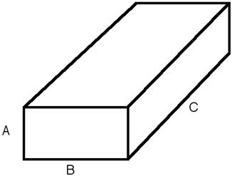
There are rectangular “slabs” of thickness \(t_A\) that add to the \(A\) dimension (on the \(BC\) faces). There are similar slabs on the \(AC\) \((=t_B)\) and \(AB\) \((=t_C)\) faces. The projection in the \(AB\) plane is then

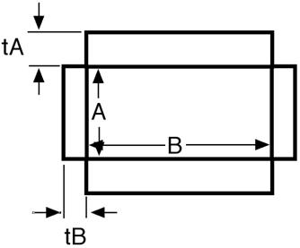
The volume of the solid is

\[V = ABC + 2t_ABC + 2t_BAC + 2t_CAB\]

meaning that there are “gaps” at the corners of the solid. Again note that \(t_C = 0\) currently.

The intensity calculated follows the parallelepiped model, with the core-shell intensity being calculated as the square of the sum of the amplitudes of the core and shell, in the same manner as a core-shell model.

Note

For the calculation of the form factor to be valid, the sides of the solid MUST be chosen such that** \(A < B < C\). If this inequality is not satisfied, the model will not report an error, but the calculation will not be correct and thus the result wrong.

FITTING NOTES If the scale is set equal to the particle volume fraction, φ, the returned value is the scattered intensity per unit volume, \(I(q) = \phi P(q)\). However, no interparticle interference effects are included in this calculation.

There are many parameters in this model. Hold as many fixed as possible with known values, or you will certainly end up at a solution that is unphysical.

Constraints must be applied during fitting to ensure that the inequality \(A < B < C\) is not violated. The calculation will not report an error, but the results will not be correct.

The returned value is in units of cm^-1, on absolute scale.

NB: The 2nd virial coefficient of the core_shell_parallelepiped is calculated based on the the averaged effective radius \((=\sqrt{(A+2t_A)(B+2t_B)/\pi})\) and length \((C+2t_C)\) values, and used as the effective radius for \(S(Q)\) when \(P(Q) * S(Q)\) is applied.

To provide easy access to the orientation of the parallelepiped, we define the axis of the cylinder using three angles \(\theta\), \(\phi\) and \(\Psi\). (see cylinder orientation). The angle \(\Psi\) is the rotational angle around the long_c axis against the \(q\) plane. For example, \(\Psi = 0\) when the short_b axis is parallel to the x-axis of the detector.

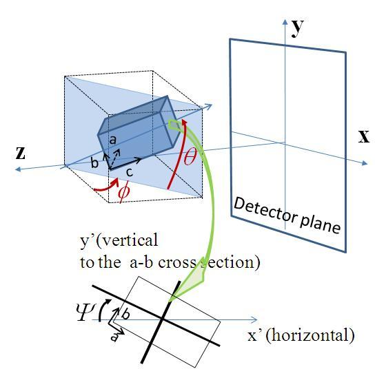
Fig. 52 Definition of the angles for oriented core-shell parallelepipeds.

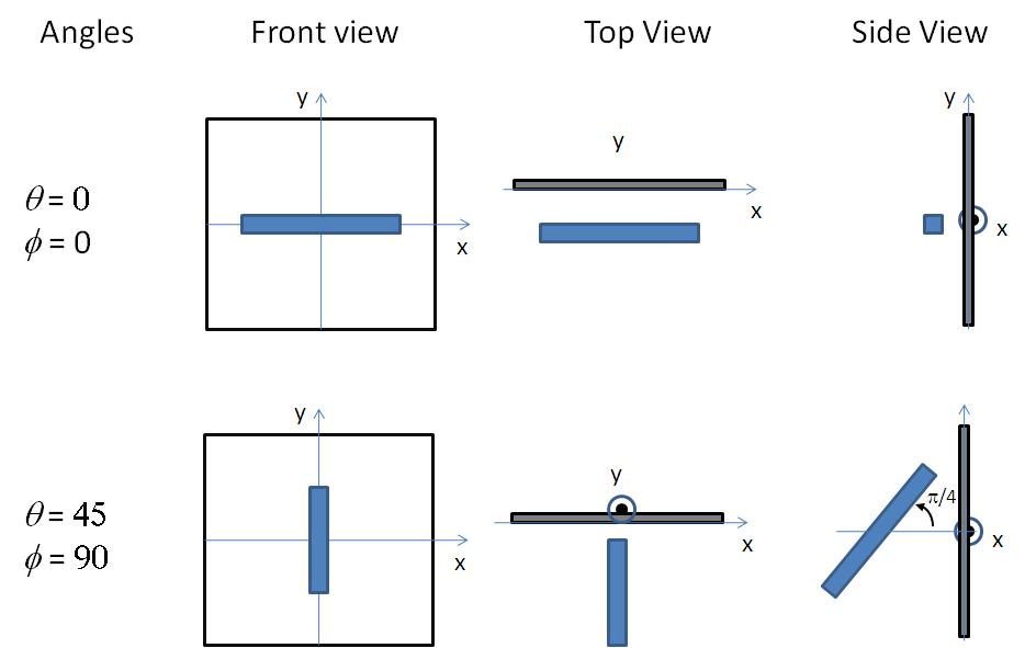
Fig. 53 Examples of the angles for oriented core-shell parallelepipeds against the detector plane.

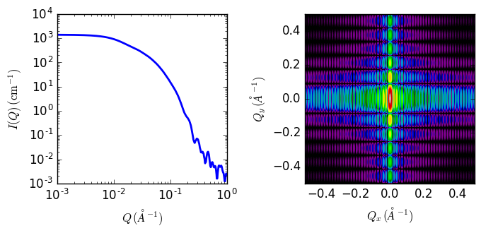
Fig. 54 1D and 2D plots corresponding to the default parameters of the model.

References

[1]	P Mittelbach and G Porod, Acta Physica Austriaca, 14 (1961) 185-211 Equations (1), (13-14). (in German)

[2]	D Singh (2009). Small angle scattering studies of self assembly in lipid mixtures, John’s Hopkins University Thesis (2009) 223-225. Available from Proquest

Authorship and Verification

• Author: NIST IGOR/DANSE Date: pre 2010
• Converted to sasmodels by: Miguel Gonzales Date: February 26, 2016
• Last Modified by: Wojciech Potrzebowski Date: January 11, 2017
• Currently Under review by: Paul Butler