parallelepiped

Rectangular parallelepiped with uniform scattering length density.

Parameter	Description	Units	Default value
scale	Source intensity	None	1
background	Source background	cm-1	0.001
sld	Parallelepiped scattering length density	10-6Å-2	4
sld_solvent	Solvent scattering length density	10-6Å-2	1
length_a	Shorter side of the parallelepiped	Å	35
length_b	Second side of the parallelepiped	Å	75
length_c	Larger side of the parallelepiped	Å	400
theta	In plane angle	degree	60
phi	Out of plane angle	degree	60
psi	Rotation angle around its own c axis against q plane	degree	60

The returned value is scaled to units of cm^-1 sr^-1, absolute scale.

The form factor is normalized by the particle volume. For information about polarised and magnetic scattering, see the Polarisation/Magnetic Scattering documentation.

Definition

This model calculates the scattering from a rectangular parallelepiped

(:numref:parallelepiped-image).

If you need to apply polydispersity, see also rectangular_prism.

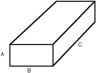
Fig. 57 Parallelepiped with the corresponding definition of sides.

Note

The edge of the solid must satisfy the condition that \(A < B < C\). This requirement is not enforced in the model, so it is up to the user to check this during the analysis.

The 1D scattering intensity \(I(q)\) is calculated as:

\[I(q) = \frac{\text{scale}}{V} (\Delta\rho \cdot V)^2 \left< P(q, \alpha) \right> + \text{background}\]

where the volume \(V = A B C\), the contrast is defined as \(\Delta\rho = \rho_\text{p} - \rho_\text{solvent}\), \(P(q, \alpha)\) is the form factor corresponding to a parallelepiped oriented at an angle \(\alpha\) (angle between the long axis C and \(\vec q\)), and the averaging \(\left<\ldots\right>\) is applied over all orientations.

Assuming \(a = A/B < 1\), \(b = B /B = 1\), and \(c = C/B > 1\), the form factor is given by (Mittelbach and Porod, 1961)

\[P(q, \alpha) = \int_0^1 \phi_Q\left(\mu \sqrt{1-\sigma^2},a\right) \left[S(\mu c \sigma/2)\right]^2 d\sigma\]

with

\[ \begin{align}\begin{aligned}\phi_Q(\mu,a) &= \int_0^1 \left\{S\left[\frac{\mu}{2}\cos\left(\frac{\pi}{2}u\right)\right] S\left[\frac{\mu a}{2}\sin\left(\frac{\pi}{2}u\right)\right] \right\}^2 du\\S(x) &= \frac{\sin x}{x}\\\mu &= qB\end{aligned}\end{align} \]

The scattering intensity per unit volume is returned in units of cm^-1.

NB: The 2nd virial coefficient of the parallelepiped is calculated based on the averaged effective radius \((=\sqrt{A B / \pi})\) and length \((= C)\) values, and used as the effective radius for \(S(q)\) when \(P(q) \cdot S(q)\) is applied.

To provide easy access to the orientation of the parallelepiped, we define three angles \(\theta\), \(\phi\) and \(\Psi\). The definition of \(\theta\) and \(\phi\) is the same as for the cylinder model (see also figures below).

The angle \(\Psi\) is the rotational angle around the \(C\) axis. For \(\theta = 0\) and \(\phi = 0\), \(\Psi = 0\) corresponds to the \(B\) axis oriented parallel to the y-axis of the detector with \(A\) along the z-axis. For other \(\theta\), \(\phi\) values, the parallelepiped has to be first rotated \(\theta\) degrees around \(z\) and \(\phi\) degrees around \(y\), before doing a final rotation of \(\Psi\) degrees around the resulting \(C\) to obtain the final orientation of the parallelepiped. For example, for \(\theta = 0\) and \(\phi = 90\), we have that \(\Psi = 0\) corresponds to \(A\) along \(x\) and \(B\) along \(y\), while for \(\theta = 90\) and \(\phi = 0\), \(\Psi = 0\) corresponds to \(A\) along \(z\) and \(B\) along \(x\).

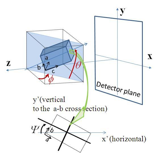
Fig. 58 Definition of the angles for oriented parallelepipeds.

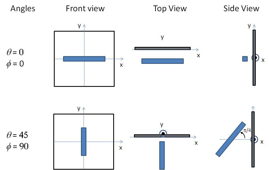
Fig. 59 Examples of the angles for oriented parallelepipeds against the detector plane.

For a given orientation of the parallelepiped, the 2D form factor is calculated as

\[P(q_x, q_y) = \left[\frac{\sin(qA\cos\alpha/2)}{(qA\cos\alpha/2)}\right]^2 \left[\frac{\sin(qB\cos\beta/2)}{(qB\cos\beta/2)}\right]^2 \left[\frac{\sin(qC\cos\gamma/2)}{(qC\cos\gamma/2)}\right]^2\]

with

\[ \begin{align}\begin{aligned}\cos\alpha &= \hat A \cdot \hat q,\\\cos\beta &= \hat B \cdot \hat q,\\\cos\gamma &= \hat C \cdot \hat q\end{aligned}\end{align} \]

and the scattering intensity as:

\[I(q_x, q_y) = \frac{\text{scale}}{V} V^2 \Delta\rho^2 P(q_x, q_y) + \text{background}\]

Validation

Validation of the code was done by comparing the output of the 1D calculation to the angular average of the output of a 2D calculation over all possible angles.

This model is based on form factor calculations implemented in a c-library provided by the NIST Center for Neutron Research (Kline, 2006).

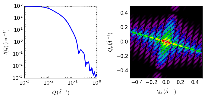
Fig. 60 1D and 2D plots corresponding to the default parameters of the model.

References

P Mittelbach and G Porod, Acta Physica Austriaca, 14 (1961) 185-211

R Nayuk and K Huber, Z. Phys. Chem., 226 (2012) 837-854