rectangular_prism

Rectangular parallelepiped with uniform scattering length density.

Parameter	Description	Units	Default value
scale	Source intensity	None	1
background	Source background	cm-1	0.001
sld	Parallelepiped scattering length density	10-6Å-2	6.3
sld_solvent	Solvent scattering length density	10-6Å-2	1
length_a	Shorter side of the parallelepiped	Å	35
b2a_ratio	Ratio sides b/a	Å	1
c2a_ratio	Ratio sides c/a	Å	1

The returned value is scaled to units of cm^-1 sr^-1, absolute scale.

This model provides the form factor, \(P(q)\), for a rectangular prism.

Note that this model is almost totally equivalent to the existing parallelepiped model. The only difference is that the way the relevant parameters are defined here ($a$, \(b/a\), \(c/a\) instead of \(a\), \(b\), \(c\)) which allows use of polydispersity with this model while keeping the shape of the prism (e.g. setting \(b/a = 1\) and \(c/a = 1\) and applying polydispersity to a will generate a distribution of cubes of different sizes). Note also that, contrary to parallelepiped, it does not compute the 2D scattering.

Definition

The 1D scattering intensity for this model was calculated by Mittelbach and Porod (Mittelbach, 1961), but the implementation here is closer to the equations given by Nayuk and Huber (Nayuk, 2012). Note also that the angle definitions used in the code and the present documentation correspond to those used in (Nayuk, 2012) (see Fig. 1 of that reference), with \(\theta\) corresponding to \(\alpha\) in that paper, and not to the usual convention used for example in the parallelepiped model. As the present model does not compute the 2D scattering, this has no further consequences.

In this model the scattering from a massive parallelepiped with an orientation with respect to the scattering vector given by \(\theta\) and \(\phi\)

\[A_P\,(q) = \frac{\sin \left( \tfrac{1}{2}qC \cos\theta \right) }{\tfrac{1}{2} qC \cos\theta} \,\times\, \frac{\sin \left( \tfrac{1}{2}qA \cos\theta \right) }{\tfrac{1}{2} qA \cos\theta} \,\times\ , \frac{\sin \left( \tfrac{1}{2}qB \cos\theta \right) }{\tfrac{1}{2} qB \cos\theta}\]

where \(A\), \(B\) and \(C\) are the sides of the parallelepiped and must fulfill \(A \le B \le C\), \(\theta\) is the angle between the \(z\) axis and the longest axis of the parallelepiped \(C\), and \(\phi\) is the angle between the scattering vector (lying in the \(xy\) plane) and the \(y\) axis.

The normalized form factor in 1D is obtained averaging over all possible orientations

\[P(q) = \frac{2}{\pi} \int_0^{\frac{\pi}{2}} \, \int_0^{\frac{\pi}{2}} A_P^2(q) \, \sin\theta \, d\theta \, d\phi\]

And the 1D scattering intensity is calculated as

\[I(q) = \text{scale} \times V \times (\rho_\text{p} - \rho_\text{solvent})^2 \times P(q)\]

where \(V\) is the volume of the rectangular prism, \(\rho_\text{p}\) is the scattering length of the parallelepiped, \(\rho_\text{solvent}\) is the scattering length of the solvent, and (if the data are in absolute units) scale represents the volume fraction (which is unitless).

The 2D scattering intensity is not computed by this model.

Validation

Validation of the code was conducted by comparing the output of the 1D model to the output of the existing parallelepiped model.

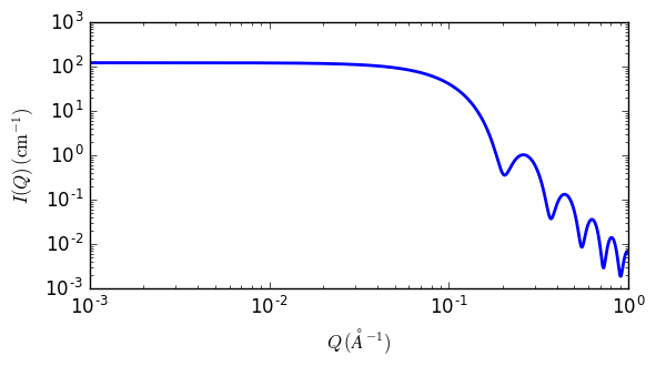
Fig. 61 1D plot corresponding to the default parameters of the model.

References

P Mittelbach and G Porod, Acta Physica Austriaca, 14 (1961) 185-211

R Nayuk and K Huber, Z. Phys. Chem., 226 (2012) 837-854