polymer_excl_volume

Polymer Excluded Volume model

Parameter	Description	Units	Default value
scale	Source intensity	None	1
background	Source background	cm-1	0.001
rg	Radius of Gyration	Å	60
porod_exp	Porod exponent	None	3

The returned value is scaled to units of cm^-1 sr^-1, absolute scale.

This model describes the scattering from polymer chains subject to excluded volume effects and has been used as a template for describing mass fractals.

Definition

The form factor was originally presented in the following integral form (Benoit, 1957)

\[P(Q)=2\int_0^{1}dx(1-x)exp\left[-\frac{Q^2a^2}{6}n^{2v}x^{2v}\right]\]

where \(\nu\) is the excluded volume parameter (which is related to the Porod exponent \(m\) as \(\nu=1/m\) ), \(a\) is the statistical segment length of the polymer chain, and \(n\) is the degree of polymerization. This integral was later put into an almost analytical form as follows (Hammouda, 1993)

\[P(Q)=\frac{1}{\nu U^{1/2\nu}}\gamma\left(\frac{1}{2\nu},U\right) - \frac{1}{\nu U^{1/\nu}}\gamma\left(\frac{1}{\nu},U\right)\]

where \(\gamma(x,U)\) is the incomplete gamma function

\[\gamma(x,U)=\int_0^{U}dt\ exp(-t)t^{x-1}\]

and the variable \(U\) is given in terms of the scattering vector \(Q\) as

\[U=\frac{Q^2a^2n^{2\nu}}{6} = \frac{Q^2R_{g}^2(2\nu+1)(2\nu+2)}{6}\]

The square of the radius-of-gyration is defined as

\[R_{g}^2 = \frac{a^2n^{2\nu}}{(2\nu+1)(2\nu+2)}\]

Note that this model applies only in the mass fractal range (ie, \(5/3<=m<=3\) ) and does not apply to surface fractals ( \(3<m<=4\) ). It also does not reproduce the rigid rod limit (m=1) because it assumes chain flexibility from the outset. It may cover a portion of the semi-flexible chain range ( \(1<m<5/3\) ).

A low-Q expansion yields the Guinier form and a high-Q expansion yields the Porod form which is given by

\[P(Q\rightarrow \infty) = \frac{1}{\nu U^{1/2\nu}}\Gamma\left( \frac{1}{2\nu}\right) - \frac{1}{\nu U^{1/\nu}}\Gamma\left( \frac{1}{\nu}\right)\]

Here \(\Gamma(x) = \gamma(x,\infty)\) is the gamma function.

The asymptotic limit is dominated by the first term

\[P(Q\rightarrow \infty) \sim \frac{1}{\nu U^{1/2\nu}}\Gamma\left(\frac{1}{2\nu}\right) = \frac{m}{\left(QR_{g}\right)^m}\left[\frac{6}{(2\nu +1)(2\nu +2)} \right]^{m/2} \Gamma (m/2)\]

The special case when \(\nu=0.5\) (or \(m=1/\nu=2\) ) corresponds to Gaussian chains for which the form factor is given by the familiar Debye function.

\[P(Q) = \frac{2}{Q^4R_{g}^4} \left[exp(-Q^2R_{g}^2) - 1 + Q^2R_{g}^2 \right]\]

For 2D data: The 2D scattering intensity is calculated in the same way as 1D, where the \(q\) vector is defined as

\[q = \sqrt{q_x^2 + q_y^2}\]

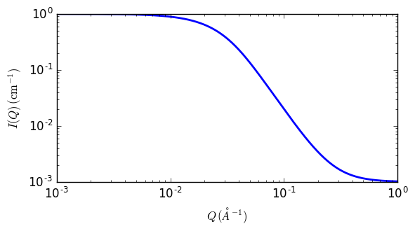
Fig. 99 1D plot corresponding to the default parameters of the model.

References

H Benoit, Comptes Rendus, 245 (1957) 2244-2247

B Hammouda, SANS from Homogeneous Polymer Mixtures - A Unified Overview, Advances in Polym. Sci. 106(1993) 87-133