raspberry
Calculates the form factor, P(q), for a ‘Raspberry-like’ structure where there are smaller spheres at the surface of a larger sphere, such as the structure of a Pickering emulsion.
Parameter |
Description |
Units |
Default value |
|---|---|---|---|
scale |
Scale factor or Volume fraction |
None |
1 |
background |
Source background |
cm-1 |
0.001 |
sld_lg |
large particle scattering length density |
10-6Å-2 |
-0.4 |
sld_sm |
small particle scattering length density |
10-6Å-2 |
3.5 |
sld_solvent |
solvent scattering length density |
10-6Å-2 |
6.36 |
volfraction_lg |
volume fraction of large spheres |
None |
0.05 |
volfraction_sm |
volume fraction of small spheres |
None |
0.005 |
surface_fraction |
fraction of small spheres at surface |
None |
0.4 |
radius_lg |
radius of large spheres |
Å |
5000 |
radius_sm |
radius of small spheres |
Å |
100 |
penetration |
fractional penetration depth of small spheres into large sphere |
Å |
0 |
The returned value is scaled to units of cm-1 sr-1, absolute scale.
Definition
The figure below shows a schematic of a large droplet surrounded by several smaller particles forming a structure similar to that of Pickering emulsions.
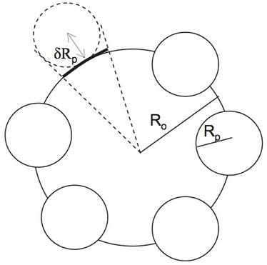
Fig. 90 Schematic of the raspberry model
In order to calculate the form factor of the entire complex, the self-correlation of the large droplet, the self-correlation of the particles, the correlation terms between different particles and the cross terms between large droplet and small particles all need to be calculated.
Consider two infinitely thin shells of radii \(R_1\) and \(R_2\) separated by distance \(r\). The general structure of the equation is then the form factor of the two shells multiplied by the phase factor that accounts for the separation of their centers.
In this case, the large droplet and small particles are solid spheres rather than thin shells. Thus the two terms must be integrated over \(R_L\) and \(R_S\) respectively using the weighting function of a sphere. We then obtain the functions for the form of the two spheres:
The cross term between the large droplet and small particles is given by:
and the self term between small particles is given by:
The number of small particles per large droplet, \(N_p\), is given by:
where \(\phi_S\) is the volume fraction of small particles in the sample, \(\phi_\text{surface}\) is the fraction of the small particles that are adsorbed to the large droplets, \(\phi_L\) is the volume fraction of large droplets in the sample, and \(V_S\) and \(V_L\) are the volumes of individual small particles and large droplets respectively.
The form factor of the entire complex can now be calculated including the excess scattering length densities of the components \(\Delta\rho_L\) and \(\Delta\rho_S\), where \(\Delta\rho_x = \left|\rho_x-\rho_\text{solvent}\right|\) :
where M is the total scattering length of the whole complex :
In a real system, there will ususally be an excess of small particles such that some fraction remain unbound. Therefore the overall scattering intensity is given by:
A useful parameter to extract is the fraction of the surface area of the large droplets that is covered by small particles. This can be calculated from the model parameters as:
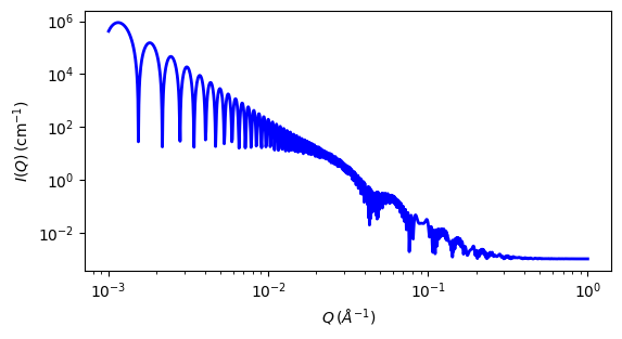
Fig. 91 1D plot corresponding to the default parameters of the model.
Source
raspberry.py
\(\ \star\ \) raspberry.c
\(\ \star\ \) sas_3j1x_x.c
References
K Larson-Smith, A Jackson, and D C Pozzo, Small angle scattering model for Pickering emulsions and raspberry particles, Journal of Colloid and Interface Science, 343(1) (2010) 36-41
Authorship and Verification
Author: Andrew Jackson Date: 2008
Last Modified by: Andrew Jackson Date: March 20, 2016
Last Reviewed by: Andrew Jackson Date: March 20, 2016