superball

Superball with uniform scattering length density.

Parameter	Description	Units	Default value
scale	Scale factor or Volume fraction	None	1
background	Source background	cm-1	0.001
sld	Superball scattering length density	10-6Å-2	4
sld_solvent	Solvent scattering length density	10-6Å-2	1
length_a	Cube edge length of the superball	Å	50
exponent_p	Exponent describing the roundness of the superball	None	2.5
theta	c axis to beam angle	degree	0
phi	rotation about beam	degree	0
psi	rotation about c axis	degree	0

The returned value is scaled to units of cm^-1 sr^-1, absolute scale.

Definition

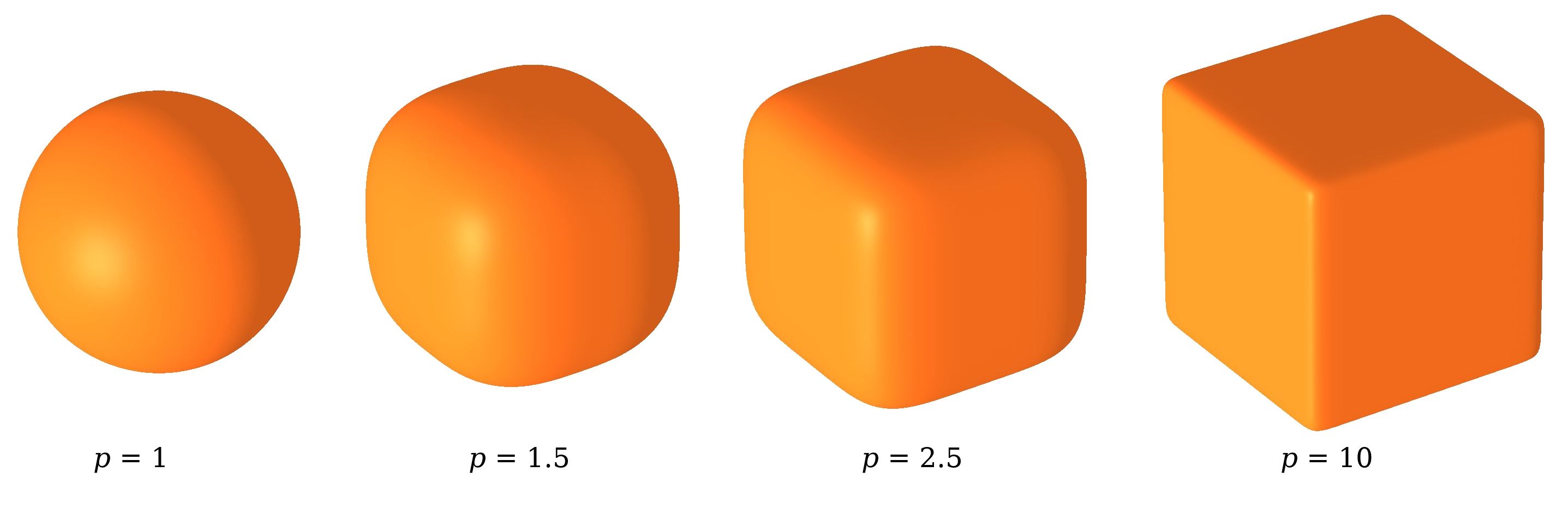
Fig. 95 Superball visualisation for varied values of the parameter p.

This model calculates the scattering of a superball, which represents a cube with rounded edges. It can be used to describe nanoparticles that deviate from the perfect cube shape as it is often observed experimentally [1]. The shape is described by

\[x^{2p} + y^{2p} + z^{2p} \leq \biggl( \frac{a}{2} \biggr)^{2p}\]

with \(a\) the cube edge length of the superball and \(p\) a parameter that describes the roundness of the edges. In the limiting cases \(p=1\) the superball corresponds to a sphere with radius \(R = a/2\) and for \(p = \infty\) to a cube with edge length \(a\). The exponent \(p\) is related to \(a\) and the face diagonal \(d\) via

\[p = \frac{1}{1 + 2 \mathrm{log}_2 (a/d)}.\]

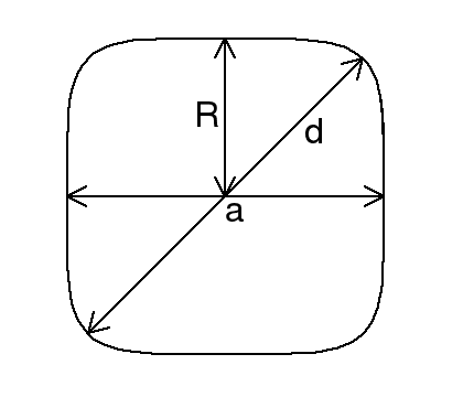
Fig. 96 Cross-sectional view of a superball showing the principal axis length \(a\), the face-diagonal \(d\) and the superball radius \(R\).

The oriented form factor is determined by solving

\[\begin{split}p_o(\vec{q}) =& \int_{V} \mathrm{d} \vec{r} e^{i \vec{q} \cdot \vec{r}}\\ =& \frac{a^3}{8} \int_{-1}^{1} \mathrm{d} x \int_{-\gamma}^{\gamma} \mathrm{d} y \int_{-\zeta}^{\zeta} \mathrm{d} z e^{i a (q_x x + q_y y + q_z z) / 2}\\ =& \frac{a^2}{2 q_z} \int_{-1}^{1} \mathrm{d} x \int_{-\gamma}^{\gamma} \mathrm{d} y e^{i a(q_x x + q_y y)/2} \sin(q_z a \zeta / 2),\end{split}\]

with

\[\begin{split}\gamma =& \sqrt[2p]{1-x^{2p}}, \\ \zeta =& \sqrt[2p]{1-x^{2p} -y^{2p}}.\end{split}\]

The integral can be transformed to

\[p_o(\vec{q}) = \frac{2 a^2}{q_z} \int_{0}^{1} \mathrm{d} x \, \cos \biggl(\frac{a q_x x}{2} \biggr) \int_{0}^{\gamma} \mathrm{d} y \, \cos \biggl( \frac{a q_y y}{2} \biggr) \sin \biggl( \frac{a q_z \zeta}{2} \biggr),\]

which can be solved numerically.

The orientational average is then obtained by calculating

\[P(q) = \int_0^{\tfrac{\pi}{2}} \mathrm{d} \varphi \int_0^{\tfrac{\pi}{2}} \mathrm{d} \theta \, \sin (\theta) | p_o(\vec{q}) |^2\]

with

\[\begin{split}\vec{q} &= q \begin{pmatrix} \cos (\varphi) \sin (\theta)\\ \sin (\varphi) \sin(\theta)\\ \cos (\theta)\end{pmatrix}\end{split}\]

The implemented orientationally averaged superball model is then fully given by [2]

\[I(q) = \mathrm{scale} (\Delta \rho)^2 P(q) + \mathrm{background}.\]

FITTING NOTES

Validation

The code is validated by reproducing the spherical form factor implemented in SasView for \(p = 1\) and the parallelepiped form factor with \(a = b = c\) for \(p = 1000\). The form factors match in the first order oscillation with a precision in the order of \(10^{-4}\). The agreement worsens for higher order oscillations and beyond the third order oscillations a higher order Gauss quadrature rule needs to be used to keep the agreement below \(10^{-3}\). This is however avoided in this implementation to keep the computation time fast.

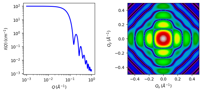
Fig. 97 1D and 2D plots corresponding to the default parameters of the model.

Source

superball.py \(\ \star\ \) superball.c \(\ \star\ \) sas_gamma.c \(\ \star\ \) gauss20.c

References

[1]

5. Wetterskog, A. Klapper, S. Disch, E. Josten, R. P. Hermann, U. Rücker, T. Brückel, L. Bergström and G. Salazar-Alvarez, Nanoscale, 8 (2016) 15571

[2]

4. Dresen, A. Qdemat, S. Ulusoy, F. Mees, D. Zakutna, E. Wetterskog, E. Kentzinger, G. Salazar-Alvarez, S. Disch, J. Phys. Chem. C (2021), doi: 10.1021/acs.jpcc.1c06082

Source

superball.py

superball.c

Authorship and Verification

• Author: Dominique Dresen Date: March 27, 2019

• Last Modified by: Dominique Dresen Date: March 27, 2019

• Last Reviewed by: Dirk Honecker Date: November 05, 2021

• Source added by : Dominique Dresen Date: March 27, 2019