hollow_rectangular_prism
Hollow rectangular parallelepiped with uniform scattering length density.
Parameter |
Description |
Units |
Default value |
|---|---|---|---|
scale |
Scale factor or Volume fraction |
None |
1 |
background |
Source background |
cm-1 |
0.001 |
sld |
Parallelepiped scattering length density |
10-6Å-2 |
6.3 |
sld_solvent |
Solvent scattering length density |
10-6Å-2 |
1 |
length_a |
Shortest, external, size of the parallelepiped |
Å |
35 |
b2a_ratio |
Ratio sides b/a |
Å |
1 |
c2a_ratio |
Ratio sides c/a |
Å |
1 |
thickness |
Thickness of parallelepiped |
Å |
1 |
theta |
c axis to beam angle |
degree |
0 |
phi |
rotation about beam |
degree |
0 |
psi |
rotation about c axis |
degree |
0 |
The returned value is scaled to units of cm-1 sr-1, absolute scale.
Definition
This model provides the form factor, \(P(q)\), for a hollow rectangular parallelepiped with a wall of thickness \(\Delta\). The 1D scattering intensity for this model is calculated by forming the difference of the amplitudes of two massive parallelepipeds differing in their outermost dimensions in each direction by the same length increment \(2\Delta\) ([1] Nayuk, 2012).
As in the case of the massive parallelepiped model (rectangular_prism), the scattering amplitude is computed for a particular orientation of the parallelepiped with respect to the scattering vector and then averaged over all possible orientations, giving
where \(\theta\) is the angle between the \(z\) axis and the \(C\) axis of the parallelepiped, \(\phi\) is the angle between the scattering vector (lying in the \(xy\) plane) and the \(y\) axis, and
\(A'\), \(B'\), \(C'\) are the inner dimensions and \(A = A' + 2\Delta\), \(B = B' + 2\Delta\), \(C = C' + 2\Delta\) are the outer dimensions of the parallelepiped shell, giving a shell volume of \(V = ABC - A'B'C'\).
The 1D scattering intensity is then calculated as
where \(\rho_\text{p}\) is the scattering length density of the parallelepiped, \(\rho_\text{solvent}\) is the scattering length density of the solvent, and (if the data are in absolute units) scale represents the volume fraction (which is unitless) of the rectangular shell of material (i.e. not including the volume of the solvent filled core).
For 2d data the orientation of the particle is required, described using angles \(\theta\), \(\phi\) and \(\Psi\) as in the diagrams below, for further details of the calculation and angular dispersions see Oriented Particles. The angle \(\Psi\) is the rotational angle around the long C axis. For example, \(\Psi = 0\) when the B axis is parallel to the x-axis of the detector.
For 2d, constraints must be applied during fitting to ensure that the inequality \(A < B < C\) is not violated, and hence the correct definition of angles is preserved. The calculation will not report an error if the inequality is not preserved, but the results may be not correct.
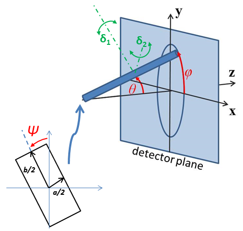
Fig. 65 Definition of the angles for oriented hollow rectangular prism. Note that rotation \(\theta\), initially in the \(xz\) plane, is carried out first, then rotation \(\phi\) about the \(z\) axis, finally rotation \(\Psi\) is now around the axis of the prism. The neutron or X-ray beam is along the \(z\) axis.
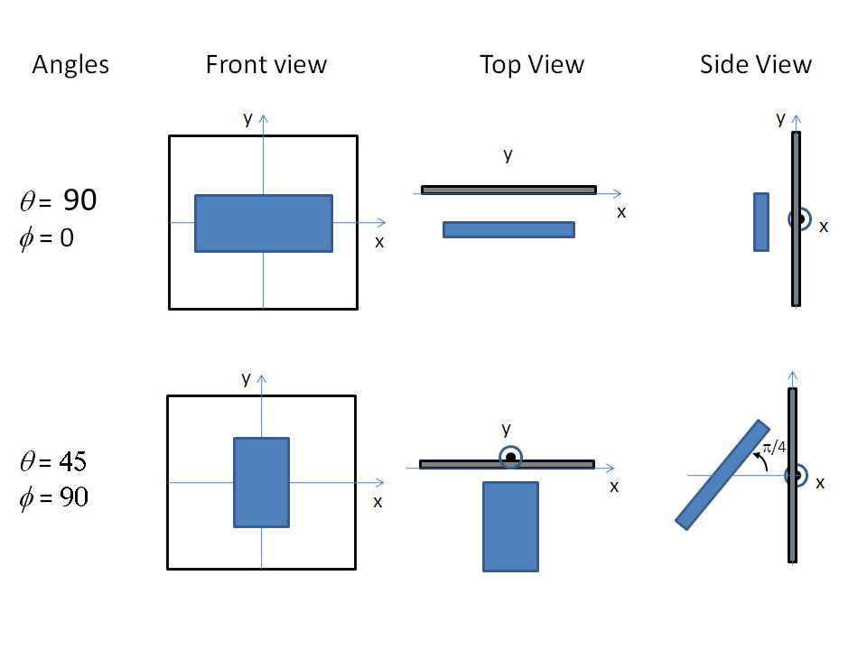
Fig. 66 Examples of the angles for oriented hollow rectangular prisms against the detector plane.
Validation
Validation of the code was conducted by qualitatively comparing the output of the 1D model to the curves shown in (Nayuk, 2012).
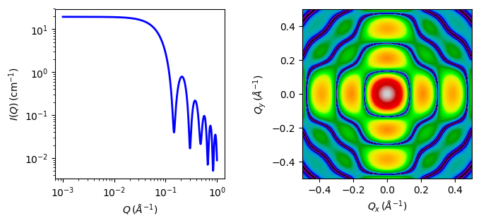
Fig. 67 1D and 2D plots corresponding to the default parameters of the model.
Source
hollow_rectangular_prism.py
\(\ \star\ \) hollow_rectangular_prism.c
\(\ \star\ \) gauss76.c
References
See also Onsager [2].
Authorship and Verification
Author: Miguel Gonzales Date: February 26, 2016
Last Modified by: Paul Kienzle Date: December 14, 2017
Last Reviewed by: Paul Butler Date: September 06, 2018